Bootstrap Confidence Intervals for 2-HT Model Parameters
Source:R/winter_2ht_boot.R
boot_winter_2ht.RdComputes bootstrap confidence intervals for the parameters of the 2-HT model by resampling the observed data with replacement.
Usage
boot_winter_2ht(
  x,
  nboot = 1000,
  conf_level = 0.95,
  lineup_size = 6,
  method = c("percentile", "bca"),
  parallel = FALSE,
  ncpus = 2,
  seed = NULL,
  ...
)
Arguments
- x
A winter_2ht object from fit_winter_2ht(), OR count data/data frame as in fit_winter_2ht().
- nboot
Number of bootstrap samples. Default is 1000.
- conf_level
Confidence level for intervals. Default is 0.95.
- lineup_size
Lineup size (only needed if x is count data, not a winter_2ht object).
- method
Type of bootstrap CI: "percentile" (default) or "bca" (bias-corrected and accelerated).
- parallel
Logical indicating whether to use parallel processing. Default is FALSE.
- ncpus
Number of CPUs to use if parallel = TRUE. Default is 2.
- seed
Random seed for reproducibility. Default is NULL.
- ...
Additional arguments passed to fit_winter_2ht().
Value
An object of class "winter_2ht_boot" containing:
- boot_estimates
Matrix of bootstrap parameter estimates (nboot x 4)
- ci
Matrix of confidence intervals for each parameter
- original_fit
The original model fit
- nboot
Number of bootstrap samples
- conf_level
Confidence level used
Details
The bootstrap procedure resamples within TP and TA strata with replacement to keep both experimental totals fixed. For each bootstrap sample, the 2-HT model is re-fitted, and the distribution of parameter estimates across bootstrap samples is used to construct confidence intervals.
Two types of confidence intervals are available:
percentile: Uses quantiles of the bootstrap distribution
bca: Bias-corrected and accelerated intervals (Efron, 1987). The bias correction counts bootstrap ties with the estimate as half, and the acceleration comes from the jackknife over individual observations, centered and scaled within TP/TA strata, using at most six distinct leave-one-out response-count fits.
References
Efron, B. (1987). Better bootstrap confidence intervals. Journal of the American Statistical Association, 82(397), 171-185.
Examples
# \donttest{
counts <- c(
n_tp_suspect = 147, n_tp_filler = 94, n_tp_reject = 141,
n_ta_suspect = 38, n_ta_filler = 138, n_ta_reject = 206
)
fit <- fit_winter_2ht(counts, lineup_size = 6)
#> Warning: 2-HT estimate is on a parameter boundary; regular Hessian standard errors are unavailable. Bootstrap intervals also need boundary qualification.
# Bootstrap CIs
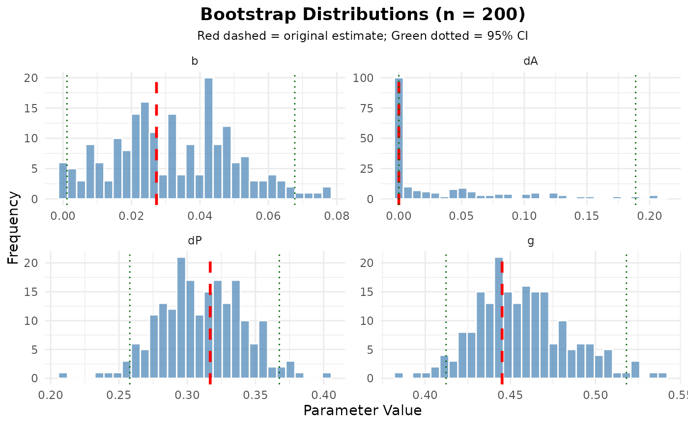
boot_fit <- boot_winter_2ht(fit, nboot = 200, seed = 123)
#> Bootstrap iteration 100/200
#> Bootstrap iteration 200/200
print(boot_fit)
#>
#> Bootstrap Confidence Intervals for 2-HT Model
#> ==============================================
#>
#> Number of bootstrap samples: 200
#> Confidence level: 95.0%
#> CI method: percentile
#>
#> Parameter Estimates with Bootstrap CIs:
#> Estimate Boot_Lower Boot_Upper Boot_SE
#> dP 0.3169 0.2580 0.3675 0.0304
#> dA 0.0000 0.0000 0.1888 0.0541
#> b 0.0273 0.0012 0.0677 0.0176
#> g 0.4452 0.4122 0.5182 0.0275
plot(boot_fit)
#> Warning: Using `size` aesthetic for lines was deprecated in ggplot2 3.4.0.
#> ℹ Please use `linewidth` instead.
#> ℹ The deprecated feature was likely used in the r4lineups package.
#> Please report the issue at <https://github.com/CGTZA2/r4lineups/issues>.
 # }