Calibration and Decision Analysis

Acknowledgement. Large language models supplied by Anthropic and OpenAI were used in preparing this vignette, to assist with checking code, testing the veracity of the approaches described, and on occasion editing the text. Responsibility for the content rests with the authors.

Introduction

This vignette demonstrates five statistical methods for analyzing eyewitness identification data in r4lineups:

Calibration Analysis - Assessing confidence-accuracy correspondence
Bayesian Information-Gain Curves - Evaluating diagnostic value of evidence
Expected Utility Analysis - Decision-theoretic evaluation with cost/benefit tradeoffs
Deviation from Perfect Performance (DPP) - ROC-based truncation-robust metric
ANRI - Bias-corrected resolution index with bootstrap inference

These methods complement the traditional lineup fairness measures by providing analyses of identification accuracy, confidence calibration, and decision-making utility.

They answer different questions.

Calibration analysis asks whether a witness’s confidence means what it appears to mean: when witnesses say they are 90% sure, are they right 90% of the time? It yields a calibration curve and three summary statistics, and it is the oldest of the five in eyewitness work (Juslin, Olsson & Winman, 1996).

Bayesian information-gain analysis asks a different question: given a particular identification response, how much should a rational observer revise their belief that the suspect is guilty? This is the framework of Wells, Yang and Smalarz (2015), and it makes explicit something the other methods leave implicit — that the evidential value of an identification depends on the prior probability of guilt, which is a property of the investigation and not of the witness.

Expected utility analysis goes one step further and asks what a policy should be. Given the costs of a wrongful identification and the benefits of a correct one, at what confidence level should an identification be acted upon? Lampinen, Smith and Wells (2019) set out the framework and show that it can disagree with ROC-based conclusions about which procedure is better.

Deviation from perfect performance (DPP) is a discriminability measure, proposed by Smith, Lampinen, Wells, Smalarz and Mackovichova (2019) as an alternative to partial area under the ROC curve. Their argument is that pAUC does not track the diagnostic utility of a lineup, and DPP does.

ANRI is a small-sample correction to the normalized resolution index. NRI (Yaniv, Yates & Smith, 1991) is positively biased when the number of confidence bins is large relative to sample size; ANRI removes that bias so that resolution can be compared across studies and tested formally.

Data Format

All methods in this vignette require a dataframe with at least the following columns:

target_present: Logical. TRUE if the guilty suspect is in the lineup
identification: Character. “suspect”, “filler”, or “reject”
confidence: Numeric. Confidence rating (any scale)

We use the built-in lineup_example dataset throughout. It contains 700 target-present and 700 target-absent lineups of size 6.

library(r4lineups)
data(lineup_example)

head(lineup_example)
  target_present lineup_member suspect_pos identification confidence
1          FALSE             2           1         filler         40
2          FALSE             3           1         filler         50
3           TRUE             2           1         filler         40
4           TRUE             1           1        suspect         80
5           TRUE             1           1        suspect         60
6          FALSE             0           1         reject         20

Why there is a `lineup_member` column

lineup_example records two further columns, for a reason that applies to any lineup data you collect or simulate yourself.

identification collapses a witness’s decision into three categories. That is what the analysis functions consume, but it is not what should be recorded. The raw datum is which lineup member the witness chose — lineup_member, with 0 for a rejection — together with the suspect’s position, suspect_pos. The label is then derived:

head(classify_lineup_choices(
  lineup_example[, c("lineup_member", "suspect_pos")],
  k = 6
))
  lineup_member suspect_pos identification
1             2           1         filler
2             3           1         filler
3             2           1         filler
4             1           1        suspect
5             1           1        suspect
6             0           1         reject

This is important because foils are not interchangeable. They differ in how plausible they are, and a foil that nobody ever chooses is not a functioning alternative to the suspect at all — it is precisely what makes a lineup unfair. Recording only “filler” throws that information away. In lineup_example the five foils attract very different numbers of choices:

lineup_table(
  lineup_example$lineup_member[lineup_example$lineup_member > 0],
  k = 6, suspect_pos = 1
)
Lineup choices (k = 6, N = 1132)

 pos:  1*    2    3    4   5   6
 cnt: 503  248  203  115  53  10

 * = nominated suspect

lineup_example is simulated, and it is simulated at the level of individual foils: each is given its own mean memory strength rather than being drawn from a common distribution. See ?simulate_lineup_data and its foil_bias argument if you want to generate data of your own on the same basis.

1. Calibration Analysis

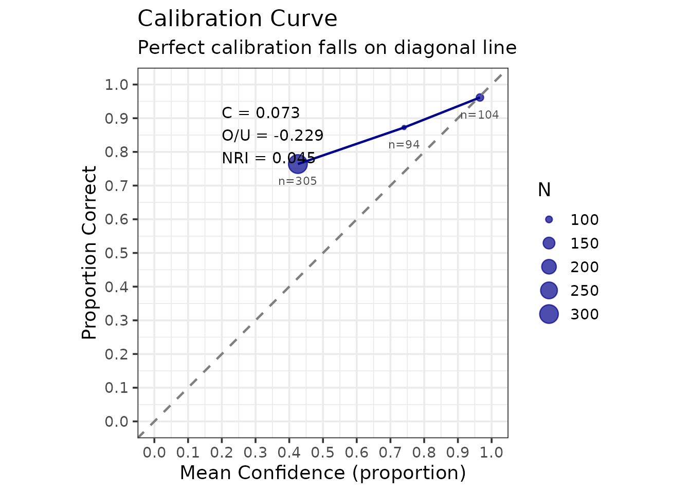
Calibration measures how well confidence judgments correspond to accuracy. Perfect calibration means that when witnesses express X% confidence, they are correct X% of the time.

Basic Calibration

# Compute calibration with binned confidence
cal_result <- make_calibration(
  lineup_example,
  confidence_bins = c(0, 60, 80, 100),
  choosers_only = TRUE  # Analyze only suspect identifications
)


print(cal_result)

=== Lineup Calibration Analysis ===

Analysis type: Choosers only (suspect IDs)
Total N: 503 

Calibration Statistics:
  C (Calibration):         0.0727 
  O/U (Over/Under):        -0.2290 
  NRI (Resolution):        0.0453 

Overall Performance:
  Mean Accuracy:      0.825 
  Mean Confidence:    0.596 

Calibration Data by Bin:
 [38;5;246m# A tibble: 3 × 7 [39m
  bin          n mean_confidence accuracy n_correct n_incorrect
   [3m [38;5;246m<chr> [39m [23m     [3m [38;5;246m<dbl> [39m [23m            [3m [38;5;246m<dbl> [39m [23m     [3m [38;5;246m<dbl> [39m [23m      [3m [38;5;246m<dbl> [39m [23m        [3m [38;5;246m<dbl> [39m [23m
 [38;5;250m1 [39m [0,60]     305            42.6    0.764       233          72
 [38;5;250m2 [39m (60,80]     94            74.0    0.872        82          12
 [38;5;250m3 [39m (80,100]   104            96.5    0.962       100           4
 [38;5;246m# ℹ 1 more variable: mean_confidence_prop <dbl> [39m

Plot: save this object first, then extract it with x$plot

The output provides three key statistics:

C statistic: Overall calibration quality (0 = perfect, higher = worse)
O/U (Over/Under confidence): Positive = overconfident, Negative = underconfident
NRI (Normalized Resolution Index): Ability to discriminate accuracy levels with confidence (higher = better)

Interpreting the Calibration Plot

The calibration plot shows:

Diagonal line: Perfect calibration
Points above diagonal: Underconfident (accuracy exceeds confidence)
Points below diagonal: Overconfident (confidence exceeds accuracy)
Point size: Sample size in each bin

cal_result$plot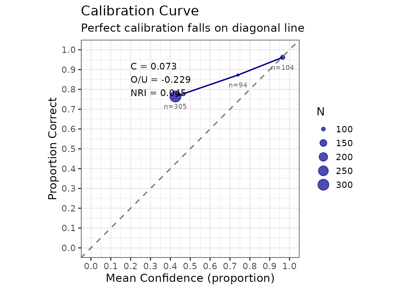

Accuracy rises steadily across the confidence bins, from about 76% in the lowest to about 96% in the highest, so confidence here is genuinely informative. The points sit above the diagonal, however, which means these witnesses are underconfident: they are more accurate than their stated confidence implies. That is the direction the O/U statistic reports.

The plot is an ordinary ggplot2 object, so it can be modified and saved in the usual way. ggsave() picks its output format from the file extension alone, so the same call writes PNG, PDF, SVG or TIFF depending on what you ask for:

outfile <- file.path(tempdir(), "calibration_plot.png")
ggplot2::ggsave(outfile, cal_result$plot, width = 8, height = 6, dpi = 300)

# Change only the extension to change the format:
#   ggsave("calibration_plot.pdf", cal_result$plot)   # vector, for print
#   ggsave("calibration_plot.svg", cal_result$plot)   # vector, for the web

Calibration by Condition

The question here is whether calibration differs between two identification procedures. To answer it we need data from two procedures, and lineup_example records only one, so we simulate them.

The comparison is only meaningful if the two conditions genuinely differ. We give Procedure A the stronger memory evidence (d_prime = 1.8 against 1.1), as might arise from better viewing conditions or a better-constructed lineup, and give the two lineups different foil quality as well. Note that both are seeded, so the results below are reproducible rather than changing on every rebuild.

# Procedure A: stronger evidence, and foils that are reasonable alternatives
data_proc_a <- as.data.frame(simulate_lineup_data(
  n_tp = 400, n_ta = 400, d_prime = 1.8, c_criterion = 0.9,
  lineup_size = 6, conf_levels = 9,
  foil_bias = c(0.4, 0.2, 0.0, -0.3, -0.8), seed = 101
))

# Procedure B: weaker evidence, and one near-useless foil
data_proc_b <- as.data.frame(simulate_lineup_data(
  n_tp = 400, n_ta = 400, d_prime = 1.1, c_criterion = 0.9,
  lineup_size = 6, conf_levels = 9,
  foil_bias = c(0.5, 0.1, -0.2, -0.9, -2.0), seed = 102
))

# Put confidence on the same 20-100 scale used by lineup_example
conf_scale <- round(seq(20, 100, length.out = 9))
data_proc_a$confidence <- conf_scale[data_proc_a$confidence]
data_proc_b$confidence <- conf_scale[data_proc_b$confidence]

# Combine into one frame with a condition variable
procedures <- rbind(
  transform(data_proc_a, procedure = "Procedure A"),
  transform(data_proc_b, procedure = "Procedure B")
)

cal_by_cond <- make_calibration_by_condition(
  procedures,
  condition_vars = "procedure",
  confidence_bins = c(0, 60, 80, 100)
)

knitr::kable(
  cal_by_cond$condition_summary, digits = 3,
  caption = "Calibration statistics by procedure, simulated data (choosers only)."
)

Calibration statistics by procedure, simulated data (choosers only).
condition	n	C	OU	NRI	overall_accuracy	overall_confidence
Procedure A	343	0.062	-0.206	0.073	0.834	0.628
Procedure B	219	0.085	-0.267	0.036	0.785	0.519

The per-bin detail for each procedure is in cal_by_cond$by_condition. The object does not carry a plot; draw one with make_calibration_by_condition_gg():

make_calibration_by_condition_gg(cal_by_cond)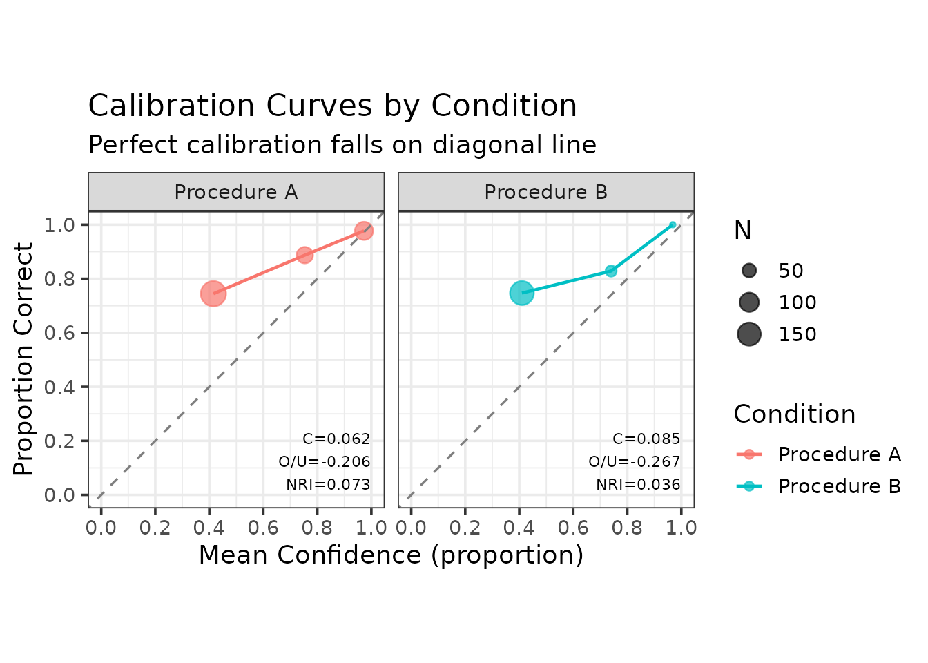

2. Bayesian Information-Gain Analysis

Bayesian analysis evaluates how much an identification response changes our belief about guilt, quantified as information gain (reduction in uncertainty). The framework is that of Wells, Yang and Smalarz (2015).

The arithmetic, briefly

Let $G$ denote the event that the suspect is guilty and $x$ a particular identification response — say, a suspect identification made with confidence above 80. Bayes’ theorem gives the posterior probability of guilt as

$P(G \mid x) \;=\; \frac{P(x \mid G)\,P(G)}{P(x \mid G)\,P(G) + P(x \mid \neg G)\,\bigl(1 - P(G)\bigr)}$

The two conditional probabilities are estimated directly from the data: $P(x \mid G)$ is the proportion of target-present witnesses who gave response $x$ , and $P(x \mid \neg G)$ the proportion of target-absent witnesses who did. Their ratio is the likelihood ratio,

$\mathrm{LR}(x) \;=\; \frac{P(x \mid G)}{P(x \mid \neg G)}$

and it is the whole of what the identification contributes. An $\mathrm{LR}$ of 1 means the response is uninformative; larger values point towards guilt, smaller towards innocence. make_bayes_curves() returns these quantities in $likelihoods:

lik <- make_bayes_curves(
  lineup_example,
  response_categories = "confidence",
  confidence_bins = c(0, 60, 80, 100)
)$likelihoods

knitr::kable(
  transform(
    as.data.frame(lik)[, c("response", "p_x_given_guilty",
                           "p_x_given_innocent", "n_guilty", "n_innocent")],
    LR = round(lik$p_x_given_guilty / lik$p_x_given_innocent, 2)
  ),
  digits = 3, row.names = FALSE,
  caption = "Response likelihoods and likelihood ratios, lineup_example."
)

Response likelihoods and likelihood ratios, lineup_example.
response	p_x_given_guilty	p_x_given_innocent	n_guilty	n_innocent	LR
filler_(60,80]	0.057	0.084	40	59	0.68
filler_(80,100]	0.019	0.043	13	30	0.43
filler_[0,60]	0.236	0.460	165	322	0.51
reject_[0,60]	0.096	0.287	67	201	0.33
suspect_(60,80]	0.117	0.017	82	12	6.83
suspect_(80,100]	0.143	0.006	100	4	25.00
suspect_[0,60]	0.333	0.103	233	72	3.24

A high-confidence suspect identification carries a likelihood ratio of roughly 25 here, while a rejection carries one of about 0.3 — that is, it is evidence against guilt. Note also that the likelihood ratio, not the posterior, is the portable quantity: it belongs to the identification procedure, whereas the posterior additionally depends on the prior, which belongs to the investigation.

One practical warning. If no target-absent witness ever produces a given response, the estimated $P(x \mid \neg G)$ is zero, the likelihood ratio is infinite, and the posterior curve is pinned at 1.0 for every prior. That is almost always a sign of too few observations or too narrow a bin rather than of perfectly diagnostic evidence, and make_bayes_curves() warns when it happens.

Prior-Posterior Curves

# Compute Bayesian curves for simple responses
bayes_result <- make_bayes_curves(
  lineup_example,
  response_categories = "simple",  # "suspect", "filler", "reject"
  prior_grid = seq(0.01, 0.99, 0.01)
)

print(bayes_result)
$curves
 [38;5;246m# A tibble: 297 × 4 [39m
   response prior posterior information_gain
    [3m [38;5;246m<chr> [39m [23m     [3m [38;5;246m<dbl> [39m [23m      [3m [38;5;246m<dbl> [39m [23m             [3m [38;5;246m<dbl> [39m [23m
 [38;5;250m 1 [39m filler    0.01   0.005 [4m3 [24m [4m3 [24m           0.032 [4m9 [24m
 [38;5;250m 2 [39m filler    0.02   0.010 [4m7 [24m            0.056 [4m0 [24m
 [38;5;250m 3 [39m filler    0.03   0.016 [4m1 [24m            0.075 [4m2 [24m
 [38;5;250m 4 [39m filler    0.04   0.021 [4m6 [24m            0.091 [4m8 [24m
 [38;5;250m 5 [39m filler    0.05   0.027 [4m2 [24m            0.106 
 [38;5;250m 6 [39m filler    0.06   0.032 [4m7 [24m            0.119 
 [38;5;250m 7 [39m filler    0.07   0.038 [4m4 [24m            0.131 
 [38;5;250m 8 [39m filler    0.08   0.044 [4m1 [24m            0.141 
 [38;5;250m 9 [39m filler    0.09   0.049 [4m8 [24m            0.151 
 [38;5;250m10 [39m filler    0.1    0.055 [4m7 [24m            0.159 
 [38;5;246m# ℹ 287 more rows [39m

$likelihoods
 [38;5;246m# A tibble: 3 × 5 [39m
  response p_x_given_guilty p_x_given_innocent n_guilty n_innocent
   [3m [38;5;246m<chr> [39m [23m                [3m [38;5;246m<dbl> [39m [23m               [3m [38;5;246m<dbl> [39m [23m     [3m [38;5;246m<int> [39m [23m       [3m [38;5;246m<dbl> [39m [23m
 [38;5;250m1 [39m filler             0.311               0.587      218        411
 [38;5;250m2 [39m reject             0.095 [4m7 [24m              0.287       67        201
 [38;5;250m3 [39m suspect            0.593               0.126      415         88

$response_counts
 [38;5;246m# A tibble: 3 × 3 [39m
  response n_guilty n_innocent
   [3m [38;5;246m<chr> [39m [23m        [3m [38;5;246m<int> [39m [23m       [3m [38;5;246m<dbl> [39m [23m
 [38;5;250m1 [39m filler        218        411
 [38;5;250m2 [39m reject         67        201
 [38;5;250m3 [39m suspect       415         88

$n_guilty
[1] 700

$n_innocent
[1] 700

$response_categories
[1] "simple"

$lineup_size
[1] 6

$innocent_suspect_method
[1] "designated"

# Plot prior-posterior relationships
plot_bayes_prior_posterior(bayes_result)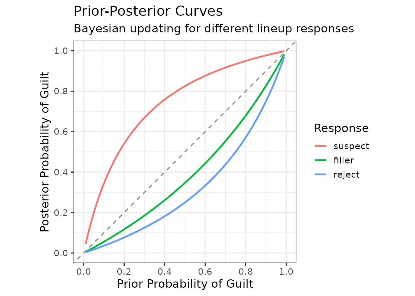

The plot shows how each response type updates prior belief:

Lines above diagonal: Evidence increases guilt belief (diagnostic of guilt)
Lines below diagonal: Evidence decreases guilt belief (diagnostic of innocence)
Distance from the diagonal: at a given prior, the further a curve lies from the diagonal, the larger the likelihood ratio of that response. Compare curves at the same prior, not by their local slopes.

The prior-posterior curve is due to Wells, Yang and Smalarz (2015), who introduced it along with the base-rate effect-equivalency curve used later in this vignette. The implementation here is written directly from that paper.

On the shape of these curves. They are curved, and that curvature is not an artefact of any smoothing: no loess or spline is fitted anywhere in these plots. For a response with likelihood ratio $L$ , the posterior as a function of the prior $p$ is $q(p) = \frac{Lp}{1 + (L - 1)p}, \qquad q''(p) = \frac{-2L(L - 1)}{[1 + (L - 1)p]^3}.$ The curvature has one sign throughout: the curve is concave (bowed above the diagonal) when $L > 1$ , convex (bowed below it) when $L < 1$ , and the diagonal itself when $L = 1$ . It is not S-shaped. What the display shows is that the same response moves belief most, in absolute terms, at middling priors, and very little when the prior is already near 0 or near 1.

Information Gain

Information gain quantifies uncertainty reduction, measured in bits: the entropy of the prior minus the entropy of the posterior. Where the posterior curve says where belief ends up, information gain says how much uncertainty was removed:

plot_bayes_information_gain(bayes_result)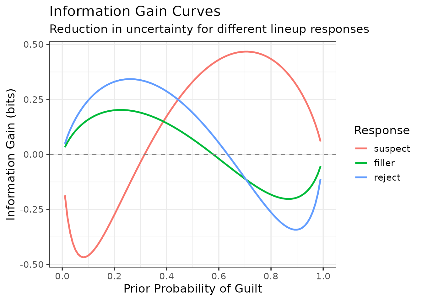

Interpretation:

Positive values: the response moves belief towards certainty (towards 0 or 1), so uncertainty falls.
Negative values: the response moves belief towards 50/50, so uncertainty rises. That is not a sign of misleading evidence: a suspect identification given a low prior raises the probability of guilt towards .5, which is the correct update and also the most uncertain state.
Where each curve peaks depends on the direction of the evidence. Responses that point to guilt (suspect identifications) gain most at priors above .5, where they push belief towards 1; responses that point to innocence (rejections, filler identifications) gain most at priors below .5.

The curves bend sharply because binary entropy changes fastest near 0 and 1. That shape is a property of the measure, not of these data or of any smoothing.

Confidence-Based Bayesian Analysis

Analyze by confidence level:

bayes_conf <- make_bayes_curves(
  lineup_example,
  response_categories = "confidence",
  confidence_bins = c(0, 60, 80, 100)
)

# Get suspect responses only
suspect_responses <- grep("^suspect_", unique(bayes_conf$curves$response), value = TRUE)
plot_bayes_prior_posterior(bayes_conf, selected_responses = suspect_responses)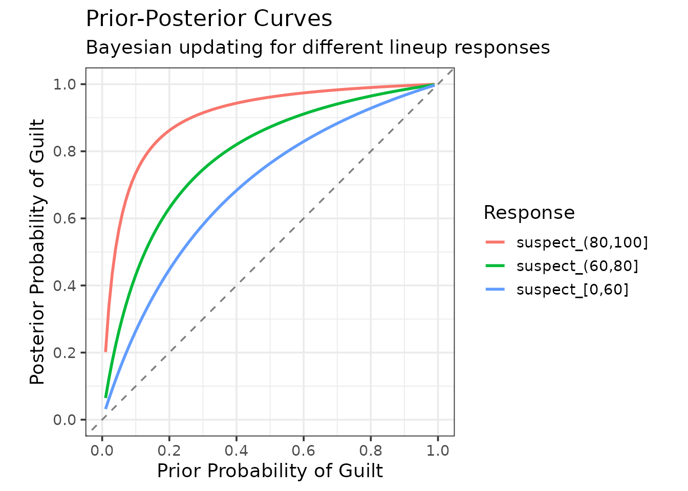

Splitting suspect identifications by confidence separates three quite different kinds of evidence. The highest-confidence band sits well above the others across the whole range of priors, which is the Bayesian restatement of the calibration result found earlier: high-confidence identifications from this procedure are worth considerably more than low-confidence ones.

The three curves stay clearly apart and none is pinned to the top of the plot. A curve that is pinned flat at 1.0 signals the zero-cell problem described above, not evidence of unusual strength.

Base-Rate Equivalency of Evidence (BREE)

The base-rate effect-equivalency curve, also from Wells, Yang and Smalarz (2015), answers a question that comes up whenever two procedures are compared and neither dominates: how much better is one than the other, expressed in units anyone can interpret?

The idea is to express the difference as an exchange rate between base rates. Suppose Procedure A, applied to a case with a 20% prior probability of guilt, yields a certain posterior after a suspect identification. We can then ask what prior Procedure B would need in order to reach that same posterior. If B needs a 40% prior to get where A got from 20%, then A is worth as much as a doubling of the base rate — and a doubling of the base rate is something an investigator has an intuition about, in a way that a difference in pAUC is not.

Plotting that correspondence for every prior gives the BREE curve. plot_bree() draws the base-rate shift $\Delta$ = prior needed by B − prior used by A, against A’s prior. The dashed horizontal line at $\Delta = 0$ is the null result of no difference; positive $\Delta$ means B needs the larger prior, so A’s suspect identification is the more diagnostic, and the further the curve lies above zero, the larger A’s advantage. (Plotting B’s prior directly against A’s would put the reference on the diagonal instead, with A’s advantage above it.)

The two procedures are the ones simulated in the Calibration by Condition section: data_proc_a and data_proc_b are data frames of target-present and target-absent identifications with confidence, one row per witness (not lineup vectors). Procedure A has the stronger memory evidence (d′ = 1.8 against 1.1).

bree_result <- make_bree_curve(
  data_proc_a,
  data_proc_b,
  reference_response = "suspect"
)

plot_bree(bree_result)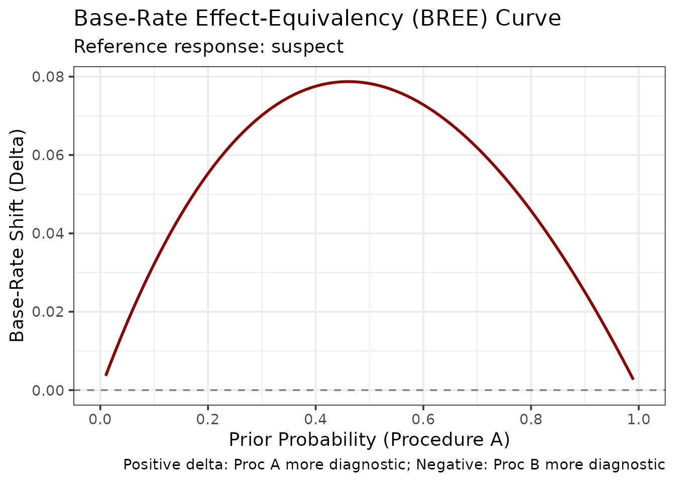

The shift is positive throughout, from 0.003 to 0.079, so Procedure B always needs a higher prior probability of guilt to reach the posterior that A reaches — which is to say that a suspect identification from Procedure A is worth more. At a prior of 0.2 for A, B needs 0.255. The shift is largest, 0.079, near a prior of 0.46, and shrinks towards both ends of the scale, where neither procedure’s evidence can move belief much.

3. Expected Utility Analysis

The methods so far describe how good a procedure is. Expected utility analysis asks what should be done about it, and it is the framework of Lampinen, Smith and Wells (2019).

The motivating observation is that discriminability measures are silent about consequences. An ROC curve treats a missed identification of a guilty suspect and the identification of an innocent one as two kinds of error, without saying how much worse one is than the other. But everyone agrees they are not equally bad, and once that is admitted, the question of which procedure is preferable cannot be settled without saying by how much. Lampinen et al. show that ROC analysis and expected utility analysis can rank the same two procedures differently — the dissociation their title refers to — so the choice of framework is not a technicality.

Define Utility Matrix

The costs and benefits must be stated explicitly. That is often felt to be the uncomfortable part of the exercise, but the values are being assumed either way; utility analysis only makes them visible and open to argument.

Four outcomes need a value, on any common scale:

utility_matrix <- c(
  tp =  1.0,   # Correct identification of a guilty suspect: a benefit
  fn = -0.5,   # Failing to identify a guilty suspect: a cost
  fp = -2.0,   # Identifying an innocent suspect: the most serious cost
  tn =  0.5    # Correctly declining to identify an innocent suspect: a benefit
)

The relative magnitudes carry the argument. Here a wrongful identification is set at four times the cost of a missed one (-2.0 against -0.5), and twice the absolute value of a correct identification’s benefit. That is a moral and legal judgement, not a statistical one, and it is the natural place for disagreement. Someone who set fp = -10 would be expressing Blackstone’s ratio; the analysis below would then recommend a considerably stricter confidence threshold. Because the choice is this important, report the sensitivity of the conclusion to it, which is what the base-rate section does for the other key assumption.

Compute Utility Curves

# Compute expected utility across confidence criteria
util_result <- make_utility_curves(
  lineup_example,
  base_rate = 0.5,  # Assume 50% guilty suspects
  utility_matrix = utility_matrix,
  lineup_size = 6
)

print(util_result)
$utility_data
 [38;5;246m# A tibble: 10 × 7 [39m
   criterion strategy   hit_rate false_alarm_rate expected_utility n_ids_tp
        [3m [38;5;246m<dbl> [39m [23m  [3m [38;5;246m<chr> [39m [23m          [3m [38;5;246m<dbl> [39m [23m             [3m [38;5;246m<dbl> [39m [23m             [3m [38;5;246m<dbl> [39m [23m     [3m [38;5;246m<dbl> [39m [23m
 [38;5;250m 1 [39m       100 threshold    0.097 [4m1 [24m          0                 0.072 [4m9 [24m       68
 [38;5;250m 2 [39m        90 threshold    0.143           0.005 [4m7 [24m [4m1 [24m           0.1         100
 [38;5;250m 3 [39m        80 threshold    0.189           0.014 [4m3 [24m            0.124       132
 [38;5;250m 4 [39m        70 threshold    0.26            0.022 [4m9 [24m            0.166       182
 [38;5;250m 5 [39m        60 threshold    0.351           0.03              0.226       246
 [38;5;250m 6 [39m        50 threshold    0.436           0.054 [4m3 [24m            0.259       305
 [38;5;250m 7 [39m        40 threshold    0.507           0.077 [4m1 [24m            0.284       355
 [38;5;250m 8 [39m        30 threshold    0.556           0.103             0.288       389
 [38;5;250m 9 [39m        20 threshold    0.593           0.126             0.288       415
 [38;5;250m10 [39m       101 reject_all   0               0                 0             0
 [38;5;246m# ℹ 1 more variable: n_ids_ta <dbl> [39m

$max_utility
$max_utility$expected_utility
       tp 
0.2882143 

$max_utility$criterion
[1] 30

$max_utility$strategy
[1] "threshold"

$max_utility$hit_rate
[1] 0.5557143

$max_utility$false_alarm_rate
[1] 0.1028571


$avg_utility
[1] 0.2008333

$utility_all_ids
    tp 
0.2875 

$base_rate
[1] 0.5

$utility_matrix
  tp   fn   fp   tn 
 1.0 -0.5 -2.0  0.5 

$n_target_present
[1] 700

$n_target_absent
[1] 700

$innocent_suspect_method
[1] "designated"

$criteria
[1] "confidence"

# Plot utility curves
plot_utility_curves(util_result)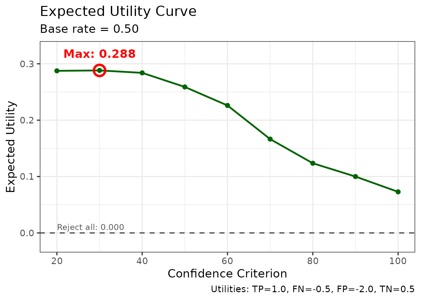

The plot shows:

Expected utility at each confidence threshold
Optimal threshold: Maximum utility point
Comparison with “all identifications” strategy

Reading it from right to left: a very strict threshold acts on almost nothing, so little is gained and little is risked. Relaxing the threshold admits identifications that are mostly correct, and utility climbs. Past the optimum, each further relaxation admits more wrongful identifications than correct ones, and because those carry four times the weight, utility falls away again. The maximum is the criterion at which the marginal identification is exactly worth acting on.

This is the shape Lampinen et al. (2019) describe. Note that the curve is usually rather flat near its peak, which is reassuring for practice: thresholds somewhat either side of the optimum lose very little, so the recommendation does not depend on locating the maximum precisely.

Compare Procedures

max_utility is a list rather than a single number: it reports the best expected utility together with the criterion that achieves it, and the hit and false-alarm rates at that criterion. Ask for the element you want.

The optimum can be a confidence criterion or the decision to reject every identification. max_utility$strategy says which, so a small helper turns the result into a rule that can be stated:

utility_rule <- function(m) {
  if (m$strategy == "reject_all") "Act on no identification"
  else paste0("Act on confidence >= ", m$criterion)
}

# Compare the two procedures simulated in the Calibration by Condition section
util_proc_a <- make_utility_curves(data_proc_a, base_rate = 0.5,
                                   utility_matrix = utility_matrix)
util_proc_b <- make_utility_curves(data_proc_b, base_rate = 0.5,
                                   utility_matrix = utility_matrix)

knitr::kable(
  data.frame(
    Procedure = c("A (d' = 1.8)", "B (d' = 1.1)"),
    `Max expected utility` = round(c(util_proc_a$max_utility$expected_utility,
                                     util_proc_b$max_utility$expected_utility), 3),
    `Optimal rule` = c(utility_rule(util_proc_a$max_utility),
                       utility_rule(util_proc_b$max_utility)),
    check.names = FALSE
  ),
  caption = "Expected utility at the optimal confidence criterion, simulated data (200 target-present and 200 target-absent lineups per procedure)."
)

Expected utility at the optimal confidence criterion, simulated data (200 target-present and 200 target-absent lineups per procedure).
Procedure	Max expected utility	Optimal rule
A (d’ = 1.8)	0.367	Act on confidence >= 40
B (d’ = 1.1)	0.185	Act on confidence >= 30

The procedure with the stronger evidence supports both a higher expected utility and a stricter criterion: it can afford to wait for high-confidence identifications because it gets more of them.

Sensitivity to Base Rate

Examine how utility depends on base rate:

# Test multiple base rates
base_rates <- c(0.2, 0.5, 0.8)

sensitivity <- do.call(rbind, lapply(base_rates, function(br) {
  util <- make_utility_curves(lineup_example, base_rate = br,
                              utility_matrix = utility_matrix,
                              lineup_size = 6)
  data.frame(
    `Base rate` = br,
    `Max expected utility` = round(util$max_utility$expected_utility, 3),
    `Optimal rule` = utility_rule(util$max_utility),
    check.names = FALSE
  )
}))

knitr::kable(
  sensitivity,
  row.names = FALSE,
  caption = "Sensitivity of expected utility to the assumed base rate, lineup_example data."
)

Sensitivity of expected utility to the assumed base rate, lineup_example data.
Base rate	Max expected utility	Optimal rule
0.2	0.345	Act on confidence >= 60
0.5	0.288	Act on confidence >= 30
0.8	0.349	Act on confidence >= 20

Base rate is very important. When guilty suspects are rare, any given identification is more likely to be a false one, so the optimal criterion becomes stricter: here “act on confidence >= 60” at a base rate of 0.2, against “act on confidence >= 20” at 0.8. The attainable utility is not ordered by base rate in any simple way, because it also depends on how the cost matrix values the outcomes that become more common; here it is 0.345, 0.288 and 0.349 at the three base rates. Compare utilities across procedures at the same base rate, not across base rates.

4. Deviation from Perfect Performance (DPP)

DPP quantifies how far an ROC curve deviates from perfect performance, and it is robust to ROC truncation — that is, to witnesses not using the full confidence scale.

It was proposed by Smith, Lampinen, Wells, Smalarz and Mackovichova (2019) as a replacement for partial area under the ROC curve, but it is contested. Lineup ROC curves cannot be traced over their full range: the observed false-alarm rate only extends as far as witnesses’ willingness to choose takes it, and that endpoint differs between procedures. pAUC handles this by integrating over a restricted region, but the choice of region is then itself a problem. Take the region from the procedure with the shorter curve and information from the other is discarded; take a common region and the comparison is made somewhere neither procedure was actually operating. Smith et al. argue that pAUC consequently fails to track which procedure has greater diagnostic utility, and that DPP does.

DPP takes a different approach. Rather than integrating over a region, it is computed at every operating point of the ROC, that is, at every cumulative confidence threshold, and then averaged. At an operating point $c$ (their Equation 2),

$DPP(c) = 1 - \text{Culprit}(c) + \text{Innocent}(c),$

where Culprit( $c$ ) is the culprit (correct) identification rate and Innocent( $c$ ) the innocent-suspect identification rate at that threshold. DPP( $c$ ) is 0 for perfect performance (every culprit identified and no innocent suspect), 1 for any point on the chance diagonal, and 2 for the worst possible performance. When culprits are present in half of all lineups and the two errors are equally costly, DPP( $c$ ) is one minus the expected utility at that threshold, so the average DPP measures the average utility of the procedure across the confidence levels witnesses actually use. Because every procedure is evaluated at its own operating points, curves of different lengths remain comparable.

This is an active disagreement rather than settled ground, and the pAUC vignette takes up the other side of it.

Basic DPP

dpp_result <- make_dpp(
  lineup_example,
  lineup_size = 6
)

dpp_result$dpp
[1] 0.7001587
dpp_result$dpp_by_point
 [38;5;246m# A tibble: 9 × 4 [39m
  confidence culprit_rate innocent_rate   dpp
        [3m [38;5;246m<dbl> [39m [23m         [3m [38;5;246m<dbl> [39m [23m          [3m [38;5;246m<dbl> [39m [23m  [3m [38;5;246m<dbl> [39m [23m
 [38;5;250m1 [39m        100       0.097 [4m1 [24m       0       0.903
 [38;5;250m2 [39m         90       0.143        0.005 [4m7 [24m [4m1 [24m 0.863
 [38;5;250m3 [39m         80       0.189        0.014 [4m3 [24m  0.826
 [38;5;250m4 [39m         70       0.26         0.022 [4m9 [24m  0.763
 [38;5;250m5 [39m         60       0.351        0.03    0.679
 [38;5;250m6 [39m         50       0.436        0.054 [4m3 [24m  0.619
 [38;5;250m7 [39m         40       0.507        0.077 [4m1 [24m  0.57 
 [38;5;250m8 [39m         30       0.556        0.103   0.547
 [38;5;250m9 [39m         20       0.593        0.126   0.533

plot_dpp(dpp_result)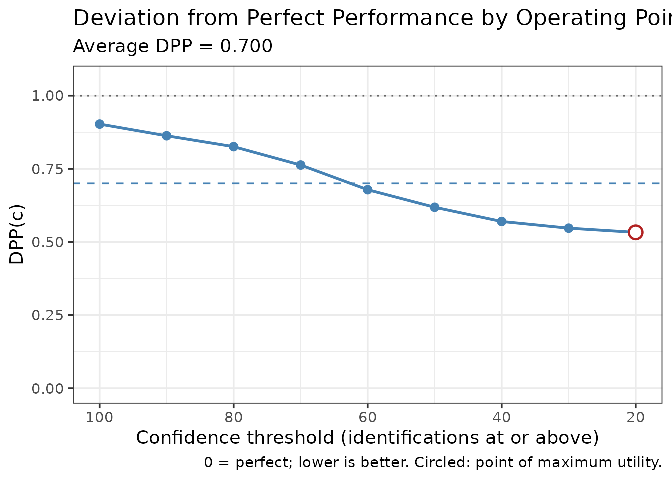

The table lists each operating point, from the strictest threshold to the most lenient, which counts every identification. The plot shows DPP( $c$ ) at each of them, the average as a dashed line, and the chance reference at 1. The circled point has the lowest DPP and so the highest utility; it is the threshold at which acting on identifications would do the most good under equal costs and a base rate of .5.

Different costs and base rates

Smith et al.’s Equation 3 weights the two errors:

$DPP_{\alpha\beta}(c) = \beta[1 - \text{Culprit}(c)] + \alpha(1 - \beta)\text{Innocent}(c),$

where $\alpha$ is the cost of identifying an innocent suspect relative to missing the culprit, and $\beta$ is the base rate of culprit presence. With $\alpha = 1$ and $\beta = .5$ this is half of Equation 2. Weighted values no longer range from 0 to 2, so they are comparable only with other values computed with the same weights.

# An innocent-suspect identification three times as costly as a miss,
# with culprits present in 30% of lineups
make_dpp(lineup_example, alpha = 3, beta = 0.3)$dpp
[1] 0.296619

Compare DPP Between Groups

The comparison is the usual use. Here the two simulated procedures from earlier differ in the strength of the evidence they generate, so Procedure A should show the smaller deviation. As Smith et al. did, compare_dpp() tests the difference with a nonparametric bootstrap, resampling target-present and target-absent trials separately within each procedure:

# Stored with the vignette; set R4LINEUPS_PRECOMPUTE=true to recompute.
dpp_comparison <- compare_dpp(
  data_proc_a,
  data_proc_b,
  lineup_size = 6,
  n_bootstrap = 500,
  seed = 2026
)

dpp_comparison

=== DPP Comparison ===

Average DPP, procedure A:  0.6022 
Average DPP, procedure B:  0.8247 
Difference (A - B):        -0.2225  (negative = A better)
Bootstrap SE:              0.0268
95% percentile interval:  [-0.2797, -0.1726]  (500 resamples)

plot_dpp_comparison(dpp_comparison)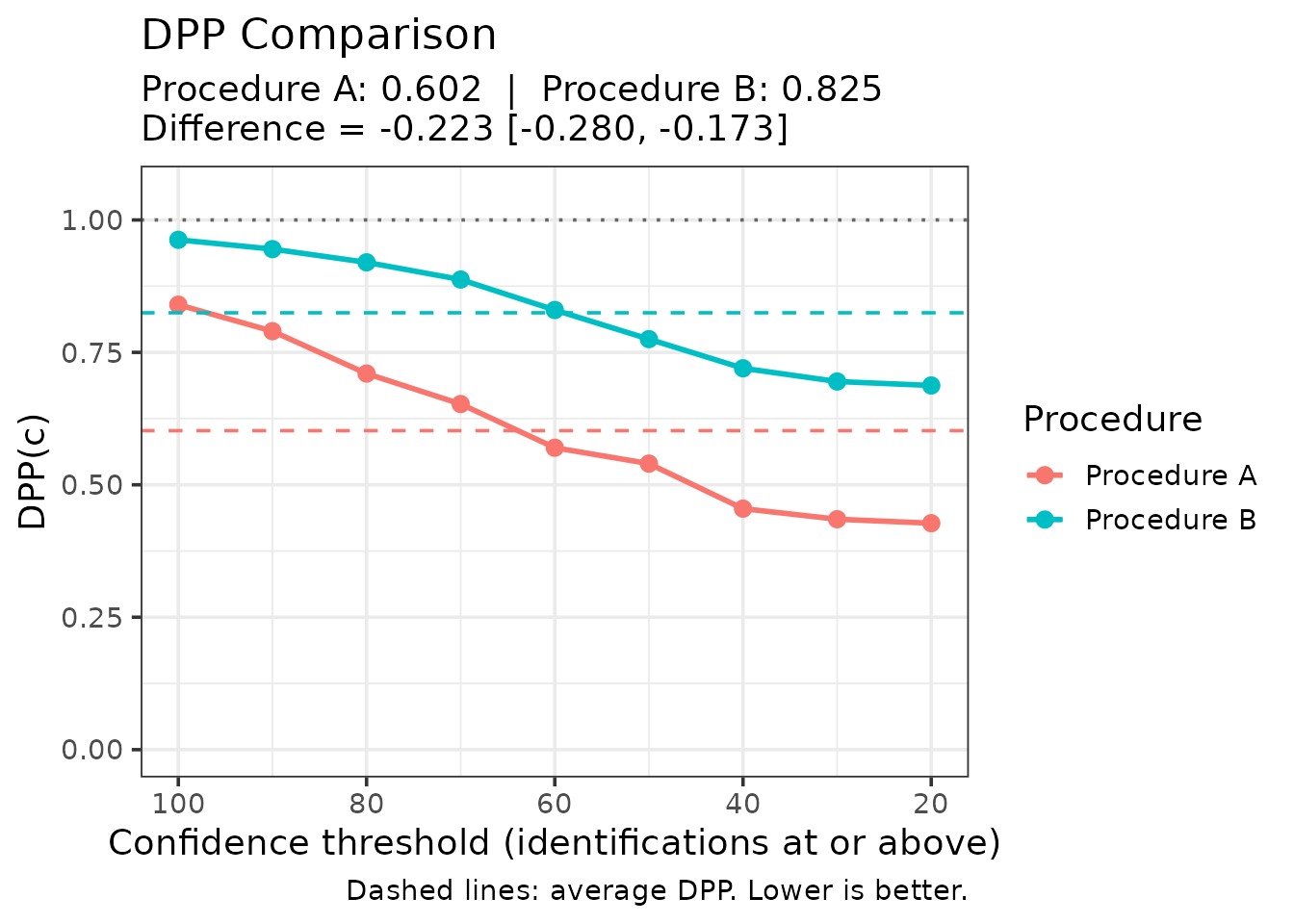

A negative difference favours Procedure A. The interval is a percentile bootstrap interval for the difference in average DPP.

When to Use DPP

Use DPP when:

You have confidence-based ROC data
ROC curves are truncated (witnesses may not use full scale)
You want a single performance metric comparable across studies
You need to compare procedures with different confidence distributions

5. ANRI: Adjusted Normalized Resolution Index

ANRI corrects NRI for small-sample bias, making it more appropriate for hypothesis testing and group comparisons.

Resolution is the third of the properties confidence can have, alongside calibration and over/underconfidence. A witness could be poorly calibrated — systematically over- or underconfident — and yet have excellent resolution, if their confidence still ranked correct identifications above incorrect ones. Resolution is arguably the most important property in practice, since a systematic bias can be corrected for once known, whereas an inability to discriminate cannot.

NRI (Yaniv, Yates & Smith, 1991) measures this, but it is positively biased: some apparent resolution arises from sampling noise alone. Splitting a sample into more confidence bins gives noise more opportunity to look like signal, so the bias grows with the number of bins and shrinks with sample size. Two studies using different numbers of bins therefore cannot have their NRIs compared directly. ANRI estimates and removes that bias.

Basic ANRI

# Compute ANRI
anri_result <- compute_anri(
  lineup_example,
  confidence_bins = c(0, 60, 80, 100)
)

print(anri_result)
$anri
[1] 0.04145948

$nri
[1] 0.04527077

$n_total
[1] 503

$n_bins
[1] 3

$calibration_data
 [38;5;246m# A tibble: 3 × 7 [39m
  bin          n mean_confidence accuracy n_correct n_incorrect
   [3m [38;5;246m<chr> [39m [23m     [3m [38;5;246m<dbl> [39m [23m            [3m [38;5;246m<dbl> [39m [23m     [3m [38;5;246m<dbl> [39m [23m      [3m [38;5;246m<dbl> [39m [23m        [3m [38;5;246m<dbl> [39m [23m
 [38;5;250m1 [39m [0,60]     305            42.6    0.764       233          72
 [38;5;250m2 [39m (60,80]     94            74.0    0.872        82          12
 [38;5;250m3 [39m (80,100]   104            96.5    0.962       100           4
 [38;5;246m# ℹ 1 more variable: mean_confidence_prop <dbl> [39m

$overall_accuracy
[1] 0.8250497

$overall_confidence
[1] 0.5960239

$choosers_only
[1] TRUE

ANRI is always ≤ NRI because it removes positive bias. The bias correction is larger when:

Sample size N is small
Number of bins J is large
The ratio J/N is high

Bootstrap Confidence Intervals

A point estimate is not much use on its own, so the interval comes from a bootstrap. n_bootstrap = 100 keeps this vignette quick; use 2000 or more for anything you intend to report.

anri_boot <- bootstrap_anri(
  lineup_example,
  confidence_bins = c(0, 60, 80, 100),
  n_bootstrap = 100,
  conf_level = 0.95,
  seed = 123
)

knitr::kable(
  data.frame(
    Statistic = c("NRI (uncorrected)", "ANRI (bias-corrected)"),
    Estimate  = round(c(anri_boot$nri, anri_boot$anri), 3),
    `95% CI`  = c("—", sprintf("[%.3f, %.3f]",
                               anri_boot$ci_lower, anri_boot$ci_upper)),
    check.names = FALSE
  ),
  row.names = FALSE,
  caption = "Resolution with bootstrap interval, lineup_example, 3 confidence bins."
)

Resolution with bootstrap interval, lineup_example, 3 confidence bins.
Statistic	Estimate	95% CI
NRI (uncorrected)	0.045	—
ANRI (bias-corrected)	0.041	[0.025, 0.068]

No interval is given for NRI because it would add nothing. ANRI is a linear rescaling of NRI, $ANRI = (N \cdot NRI - J + 1)/(N - J + 1)$ , so with $N =$ 503 suspect identifications and $J =$ 3 bins the two differ only by the bias correction (0.045 against 0.041 here). An interval for NRI would be the ANRI interval shifted upward by that bias, so it is ANRI and its interval that should be reported and compared.

Compare Groups

The comparison uses the two simulated procedures, which differ in the strength of the evidence they generate. Because they were simulated with genuinely different parameters, any difference found here reflects that design rather than chance group assignment.

anri_comparison <- compare_anri(
  procedures,
  group_var = "procedure",
  confidence_bins = c(0, 60, 80, 100),
  n_bootstrap = 100,
  seed = 456
)

print(anri_comparison)
$anri_group1
[1] 0.06778469

$anri_group2
[1] 0.02682759

$nri_group1
[1] 0.07322035

$nri_group2
[1] 0.03571501

$difference
[1] 0.04095711

$ci_lower
[1] -0.0162656

$ci_upper
[1] 0.09288628

$conf_level
[1] 0.95

$significant
 2.5% 
FALSE 

$group_names
[1] "Procedure A" "Procedure B"

$n_bootstrap
[1] 100

$n_bootstrap_requested
[1] 100

$n_failed
[1] 0

$bootstrap_results_group1
$bootstrap_results_group1$anri
[1] 0.06778469

$bootstrap_results_group1$nri
[1] 0.07322035

$bootstrap_results_group1$ci_lower
[1] 0.02912137

$bootstrap_results_group1$ci_upper
[1] 0.1149089

$bootstrap_results_group1$conf_level
[1] 0.95

$bootstrap_results_group1$n_bootstrap
[1] 100

$bootstrap_results_group1$n_bootstrap_requested
[1] 100

$bootstrap_results_group1$n_failed
[1] 0

$bootstrap_results_group1$n_total
[1] 343

$bootstrap_results_group1$n_bins
[1] 3

$bootstrap_results_group1$bootstrap_distribution
  [1] 0.06708598 0.06570604 0.08047661 0.04987933 0.07221240 0.06148205
  [7] 0.07212585 0.08571190 0.06816675 0.06999423 0.05916390 0.09510135
 [13] 0.03142914 0.04505713 0.05639861 0.09915104 0.03885619 0.07716533
 [19] 0.05518367 0.06160329 0.08011800 0.03582855 0.05369086 0.08262844
 [25] 0.11270127 0.09078520 0.11118346 0.06107025 0.11095935 0.03686786
 [31] 0.07824433 0.10365266 0.06466421 0.07758830 0.06246753 0.04141894
 [37] 0.08328425 0.08469806 0.08008407 0.06726736 0.02703340 0.06715568
 [43] 0.06081143 0.04384714 0.06404480 0.08060125 0.09375399 0.04073706
 [49] 0.05561147 0.06537103 0.08259529 0.07587945 0.06234151 0.11957211
 [55] 0.06314098 0.02570420 0.04332888 0.09238761 0.10012490 0.11869072
 [61] 0.05276179 0.09538591 0.07677354 0.04634813 0.08990006 0.05857359
 [67] 0.10507931 0.07623093 0.11105741 0.07602279 0.08272019 0.04113382
 [73] 0.08082205 0.05360715 0.09284835 0.01839824 0.03796410 0.07069711
 [79] 0.07777091 0.08588510 0.11690619 0.06030880 0.10590118 0.10782745
 [85] 0.06639759 0.06499843 0.07933454 0.06463416 0.09112998 0.06640864
 [91] 0.06755599 0.07182240 0.09123954 0.07012033 0.09326807 0.08488978
 [97] 0.08600358 0.07038152 0.06785717 0.03480324


$bootstrap_results_group2
$bootstrap_results_group2$anri
[1] 0.02682759

$bootstrap_results_group2$nri
[1] 0.03571501

$bootstrap_results_group2$ci_lower
[1] 0.009110349

$bootstrap_results_group2$ci_upper
[1] 0.06445527

$bootstrap_results_group2$conf_level
[1] 0.95

$bootstrap_results_group2$n_bootstrap
[1] 100

$bootstrap_results_group2$n_bootstrap_requested
[1] 100

$bootstrap_results_group2$n_failed
[1] 0

$bootstrap_results_group2$n_total
[1] 219

$bootstrap_results_group2$n_bins
[1] 3

$bootstrap_results_group2$bootstrap_distribution
  [1] 0.054817973 0.022421218 0.026550014 0.047942448 0.026436048 0.051313022
  [7] 0.026715655 0.035606414 0.049266532 0.033202453 0.065100176 0.019272279
 [13] 0.017972351 0.024914903 0.031759105 0.023415879 0.039935663 0.016485797
 [19] 0.028106056 0.026755049 0.042393733 0.014044901 0.047430438 0.025694351
 [25] 0.009603482 0.031974042 0.025750449 0.023649520 0.016634482 0.034929618
 [31] 0.044207564 0.042362668 0.025991477 0.033185154 0.037640835 0.026160620
 [37] 0.011972828 0.007036663 0.041360143 0.024607043 0.027630872 0.030317349
 [43] 0.032542761 0.019641566 0.022733987 0.010714669 0.031485628 0.021524720
 [49] 0.021008661 0.029182388 0.023620195 0.032096170 0.032127258 0.039164861
 [55] 0.022085988 0.045748433 0.022176174 0.023266895 0.034157548 0.023283074
 [61] 0.064850996 0.008664181 0.014826744 0.024504903 0.010977051 0.019082504
 [67] 0.013783056 0.023553399 0.032484769 0.026147752 0.022248487 0.030642495
 [73] 0.007978659 0.057524655 0.027271420 0.064017894 0.080392203 0.014551924
 [79] 0.051559618 0.026730444 0.026491746 0.023184755 0.035857128 0.028955733
 [85] 0.019554188 0.048800873 0.022485638 0.034746265 0.046738180 0.030777372
 [91] 0.026480496 0.025514253 0.037440071 0.038654235 0.034623890 0.033019727
 [97] 0.053811990 0.030239350 0.028706437 0.010009702


$difference_distribution
  [1]  0.0122680065  0.0432848222  0.0539265958  0.0019368818  0.0457763559
  [6]  0.0101690294  0.0454101932  0.0501054840  0.0189002169  0.0367917783
 [11] -0.0059362774  0.0758290756  0.0134567857  0.0201422261  0.0246395094
 [16]  0.0757351573 -0.0010794705  0.0606795334  0.0270776135  0.0348482420
 [21]  0.0377242712  0.0217836462  0.0062604171  0.0569340862  0.1030977881
 [26]  0.0588111547  0.0854330116  0.0374207301  0.0943248658  0.0019382433
 [31]  0.0340367627  0.0612899930  0.0386727321  0.0444031450  0.0248266917
 [36]  0.0152583218  0.0713114246  0.0776613940  0.0387239227  0.0426603164
 [41] -0.0005974759  0.0368383268  0.0282686652  0.0242055779  0.0413108181
 [46]  0.0698865853  0.0622683605  0.0192123438  0.0346028060  0.0361886426
 [51]  0.0589750985  0.0437832779  0.0302142505  0.0804072525  0.0410549946
 [56] -0.0200442308  0.0211527091  0.0691207197  0.0659673547  0.0954076458
 [61] -0.0120892085  0.0867217281  0.0619467959  0.0218432288  0.0789230117
 [66]  0.0394910885  0.0912962539  0.0526775336  0.0785726379  0.0498750399
 [71]  0.0604717015  0.0104913202  0.0728433901 -0.0039175017  0.0655769263
 [76] -0.0456196567 -0.0424281019  0.0561451813  0.0262112892  0.0591546516
 [81]  0.0904144437  0.0371240484  0.0700440502  0.0788717134  0.0468434025
 [86]  0.0161975531  0.0568489007  0.0298878990  0.0443917958  0.0356312668
 [91]  0.0410754920  0.0463081431  0.0537994645  0.0314660929  0.0586441834
 [96]  0.0518700487  0.0321915922  0.0401421675  0.0391507322  0.0247935330

plot_anri_comparison(anri_comparison)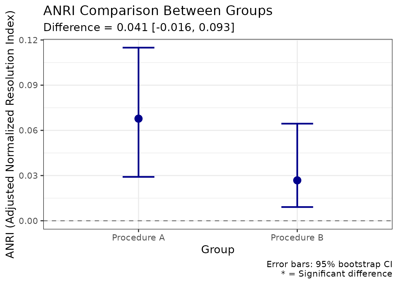

The comparison provides:

Point estimates for each group
Difference with CI: Tests whether groups differ
Significance test: CI excludes 0 = significant difference

The bootstrap difference distribution is available as plot_anri_difference_distribution(anri_comparison) if you want to inspect its shape. Inspect it when an interval looks surprising: a heavily skewed or multimodal distribution is a sign the bins are too thin somewhere.

When to Use ANRI vs NRI

The considerations, rather than rules:

ANRI is the safer default whenever the bias it corrects could be material — modest samples (say a few hundred or fewer), several confidence bins, or any comparison across studies that binned confidence differently. Because the bias grows with the bin-to-sample ratio, it is exactly the studies most likely to be compared informally that are least comparable on raw NRI. Formal tests should use ANRI, since testing a biased estimate against zero tests the wrong thing.

NRI remains reasonable when the correction is negligible — large samples with few bins, where ANRI and NRI will agree closely anyway — or when the point is to compare with older published work that reported NRI. In the analysis above the two differ by very little, which is what a sample of this size should produce.

Reporting both, as the table above does, costs nothing and lets a reader see the size of the correction for themselves.

Integrating Multiple Methods

For a comprehensive analysis, combine these methods:

Each method answers a different question, so a full analysis runs several. The five calls below use lineup_example; substitute your own data frame.

bins <- c(0, 60, 80, 100)

# 1. Calibration: does confidence mean what it says?
cal <- make_calibration(lineup_example, confidence_bins = bins,
                        show_plot = FALSE)

# 2. DPP: average utility across operating points
dpp <- make_dpp(lineup_example, lineup_size = 6)

# 3. ANRI: resolution, with inference
anri <- bootstrap_anri(lineup_example, confidence_bins = bins,
                       n_bootstrap = 100, seed = 789)

# 4. Utility: what should be done about it?
util <- make_utility_curves(lineup_example, base_rate = 0.5,
                            utility_matrix = utility_matrix,
                            lineup_size = 6)

# 5. Bayesian: what is an identification worth as evidence?
bayes <- make_bayes_curves(lineup_example, response_categories = "confidence",
                           confidence_bins = bins)

knitr::kable(
  data.frame(
    Method   = c("Calibration (C)", "Over/underconfidence (O/U)",
                 "DPP", "ANRI", "Max expected utility"),
    Estimate = round(c(cal$C, cal$OU, dpp$dpp, anri$anri,
                       util$max_utility$expected_utility), 3)
  ),
  row.names = FALSE,
  caption = "Summary across all five methods, lineup_example."
)

Summary across all five methods, lineup_example.
Method	Estimate
Calibration (C)	0.073
Over/underconfidence (O/U)	-0.229
DPP	0.700
ANRI	0.041
Max expected utility	0.288

Reporting Results

Example Write-Up

Every number below is computed from the objects created above rather than typed in, so this passage cannot drift out of step with the analysis it describes. The same practice suits a manuscript.

We analysed identification performance using calibration analysis, deviation from perfect performance (DPP), and the adjusted normalized resolution index (ANRI) with bootstrap inference, using 1400 lineups of size 6 (700 target-present, 700 target-absent).

Witnesses were well calibrated overall (C = 0.073), but systematically underconfident (O/U = -0.229): accuracy in the lowest confidence band was substantially higher than stated confidence implied. Average DPP was 0.7 (0 = perfect, 1 = chance), and the operating point of maximum utility was confidence of 20 or above (DPP = 0.533). Resolution, measured by ANRI, was 0.041 (95% CI [0.021, 0.072]), against an uncorrected NRI of 0.045.

Expected utility analysis assumed a base rate of 50% and the cost matrix u(correct suspect ID) = 1, u(missed guilty suspect) = -0.5, u(innocent suspect ID) = -2, u(correct rejection) = 0.5; that is, a wrongful identification was weighted four times as heavily as a missed one. Under those assumptions the rule “act on confidence >= 30” maximised expected utility (EU = 0.288).

Bayesian analysis showed that high-confidence suspect identifications were the most informative response, with a likelihood ratio of 25 (based on 100 guilty-suspect and 4 innocent-suspect identifications in that band).

Note the last parenthesis. The likelihood ratio there rests on very few target-absent observations, and reporting the counts alongside the ratio is what allows a reader to judge how much weight it will bear.

References

Brewer, N., & Wells, G. L. (2006). The confidence-accuracy relationship in eyewitness identification: Effects of lineup instructions, foil similarity, and target-absent base rates. Journal of Experimental Psychology: Applied, 12(1), 11-30.

Juslin, P., Olsson, N., & Winman, A. (1996). Calibration and diagnosticity of confidence in eyewitness identification: Comments on what can be inferred from the low confidence-accuracy correlation. Journal of Experimental Psychology: Learning, Memory, and Cognition, 22(5), 1304-1316.

Lampinen, J. M., Smith, A. M., & Wells, G. L. (2019). Four utilities in eyewitness identification practice: Dissociations between receiver operating characteristic (ROC) analysis and expected utility analysis. Law and Human Behavior, 43(1), 26-44.

Mickes, L. (2015). Receiver operating characteristic analysis and confidence-accuracy characteristic analysis in investigations of system variables and estimator variables that affect eyewitness memory. Journal of Applied Research in Memory and Cognition, 4(2), 93-102.

Smith, A. M., Lampinen, J. M., Wells, G. L., Smalarz, L., & Mackovichova, S. (2019). Deviation from perfect performance measures the diagnostic utility of eyewitness lineups but partial area under the ROC curve does not. Journal of Applied Research in Memory and Cognition, 8(1), 50-59. https://doi.org/10.1016/j.jarmac.2018.09.003

Wells, G. L., Yang, Y., & Smalarz, L. (2015). Eyewitness identification: Bayesian information gain, base-rate effect-equivalency curves, and reasonable suspicion. Law and Human Behavior, 39(2), 99-122.

Yaniv, I., Yates, J. F., & Smith, J. E. K. (1991). Measures of discrimination skill in probabilistic judgment. Psychological Bulletin, 110(3), 611-617.

Session Info

sessionInfo()
R version 4.6.2 (2026-10-29)
Platform: x86_64-pc-linux-gnu
Running under: Ubuntu 26.04.1 LTS

Matrix products: default
BLAS:   /usr/lib/x86_64-linux-gnu/openblas-pthread/libblas.so.3 
LAPACK: /usr/lib/x86_64-linux-gnu/openblas-pthread/libopenblasp-r0.3.32.so;  LAPACK version 3.12.0

locale:
 [1] LC_CTYPE=C.UTF-8       LC_NUMERIC=C           LC_TIME=C.UTF-8       
 [4] LC_COLLATE=C.UTF-8     LC_MONETARY=C.UTF-8    LC_MESSAGES=C.UTF-8   
 [7] LC_PAPER=C.UTF-8       LC_NAME=C              LC_ADDRESS=C          
[10] LC_TELEPHONE=C         LC_MEASUREMENT=C.UTF-8 LC_IDENTIFICATION=C   

time zone: UTC
tzcode source: system (glibc)

attached base packages:
[1] stats     graphics  grDevices utils     datasets  methods   base     

other attached packages:
[1] r4lineups_2.3.0

loaded via a namespace (and not attached):
 [1] Matrix_1.7-6       gtable_0.3.6       jsonlite_2.0.0     dplyr_1.2.1       
 [5] compiler_4.6.2     tidyselect_1.2.1   Rcpp_1.1.2         gridExtra_2.3.1   
 [9] jquerylib_0.1.4    png_0.1-9          systemfonts_1.3.2  scales_1.4.0      
[13] textshaping_1.0.5  boot_1.3-32        yaml_2.3.12        fastmap_1.2.0     
[17] lattice_0.23-1     reticulate_1.47.0  ggplot2_4.0.3      R6_2.6.1          
[21] labeling_0.4.3     generics_0.1.4     knitr_1.52         htmlwidgets_1.6.4 
[25] ggrepel_0.9.8      tibble_3.3.1       desc_1.4.3         bslib_0.12.0      
[29] pillar_1.11.1      RColorBrewer_1.1-3 rlang_1.3.0        utf8_1.2.6        
[33] cachem_1.1.0       xfun_0.62          fs_2.1.0           sass_0.4.10       
[37] S7_0.2.2           otel_0.2.0         cli_3.6.6          withr_3.0.3       
[41] pkgdown_2.2.1      magrittr_2.0.5     digest_0.6.39      grid_4.6.2        
[45] lifecycle_1.0.5    vctrs_0.7.3        evaluate_1.0.5     glue_1.8.1        
[49] farver_2.1.2       ragg_1.5.2         purrr_1.2.2        rmarkdown_2.32    
[53] tools_4.6.2        pkgconfig_2.0.3    htmltools_0.5.9

Advanced Methods for Evaluating Eyewitness Identification Performance

Colin G. Tredoux

Tamsyn M. Naylor

2026-11-02

Introduction

Data Format

Why there is a `lineup_member` column

1. Calibration Analysis

Basic Calibration

Interpreting the Calibration Plot

Calibration by Condition

2. Bayesian Information-Gain Analysis

The arithmetic, briefly

Prior-Posterior Curves

Information Gain

Confidence-Based Bayesian Analysis

Base-Rate Equivalency of Evidence (BREE)

3. Expected Utility Analysis

Define Utility Matrix

Compute Utility Curves

Compare Procedures

Sensitivity to Base Rate

4. Deviation from Perfect Performance (DPP)

Basic DPP

Different costs and base rates

Compare DPP Between Groups

When to Use DPP

5. ANRI: Adjusted Normalized Resolution Index

Basic ANRI

Bootstrap Confidence Intervals

Compare Groups

When to Use ANRI vs NRI

Integrating Multiple Methods

Reporting Results

Example Write-Up

References

Session Info

Calibration and Decision Analysis

Advanced Methods for Evaluating Eyewitness Identification Performance

Colin G. Tredoux

Tamsyn M. Naylor

2026-11-02

Introduction

Data Format

Why there is a lineup_member column

1. Calibration Analysis

Basic Calibration

Interpreting the Calibration Plot

Calibration by Condition

2. Bayesian Information-Gain Analysis

The arithmetic, briefly

Prior-Posterior Curves

Information Gain

Confidence-Based Bayesian Analysis

Base-Rate Equivalency of Evidence (BREE)

3. Expected Utility Analysis

Define Utility Matrix

Compute Utility Curves

Compare Procedures

Sensitivity to Base Rate

4. Deviation from Perfect Performance (DPP)

Basic DPP

Different costs and base rates

Compare DPP Between Groups

When to Use DPP

5. ANRI: Adjusted Normalized Resolution Index

Basic ANRI

Bootstrap Confidence Intervals

Compare Groups

When to Use ANRI vs NRI

Integrating Multiple Methods

Reporting Results

Example Write-Up

References

Session Info

Why there is a `lineup_member` column