RAC Analysis: Response Time-Accuracy Characteristics

Acknowledgement. Large language models supplied by Anthropic and OpenAI were used in preparing this vignette, to assist with checking code, testing the veracity of the approaches described, and on occasion editing the text. Responsibility for the content rests with the authors.

Introduction

This vignette demonstrates RAC (Response Time-Accuracy Characteristic) analysis for eyewitness lineup data.

The RAC plot is recent, and the implementation here follows pyWitness (Mickes et al., 2024). The underlying idea is not recent at all. That identification accuracy is related to how long a witness takes to decide has been an active research question since at least the early 1990s: Sporer (1993) reported that decision times for correct identifications were shorter than for incorrect ones, and used decision time along with confidence to postdict accuracy. What RAC adds is a display that puts response time on the same footing as the CAC plot puts confidence, not a new finding.

Why response time?

Fast responses often indicate strong memory. The intuition is that a strong memory produces recognition that feels automatic — the face is recognised rather than worked out by comparing candidates one against another. This is related to Tulving’s notion of ecphory, the process by which a retrieval cue contacts a stored trace and produces the experience of remembering; a strong trace yields an immediate ecphoric experience, a weak one yields deliberation. Dunning and Perretta (2002) made the automaticity version of this argument explicitly.
Response time is objective. Unlike confidence, it is recorded rather than reported, so it is less exposed to post-event influence and to feedback from the lineup administrator.
Complementary to confidence. RAC and CAC together may give a fuller picture than either alone.
Forensically practical. Response time can be captured automatically in video and computer-administered lineups at no cost to the witness.

The 10-to-12-second rule, and what happened to it

Any discussion of response time in this area has to deal with the best-known claim about it. Dunning and Perretta (2002) reported that a boundary of roughly 10 to 12 seconds separated accurate from inaccurate positive identifications: witnesses deciding faster than that were close to 90% accurate, those taking longer around 50%.

The rule did not survive replication. Weber, Brewer, Wells, Semmler and Keast (2004) analysed a large set of studies and found that although accurate identifications were indeed faster than inaccurate ones, the boundary that best separated them varied enormously between experiments — from about 5 seconds to about 29 seconds. There is a real speed-accuracy relationship; there is no universal number.

The practical consequence shapes how this vignette proceeds. A time boundary should be estimated from the data in hand rather than imported from another study. The continuous approach below does that. It gives a point estimate of the boundary; an interval for the boundary itself would need a further step, such as bootstrapping the whole fit, which this vignette does not show.

Setup

library(r4lineups)
library(ggplot2)

Simulating Data with Response Times

Few existing datasets include response times, so we simulate. The choices are generated by simulate_lineup_data(), which draws a memory strength for every lineup member separately and gives each foil its own mean via foil_bias, so the foils are not interchangeable.

Response times are then added by an explicit model: time falls as the strength of the evidence rises, plus noise. This part is a construction, not a simulation of any published finding, and the noise is set so that the correlation between response time and confidence is moderate — about −0.5 — rather than the near-perfect relationship that would make the demonstration trivial.

set.seed(123)

lineup_data <- as.data.frame(simulate_lineup_data(
  n_tp = 600, n_ta = 600,
  d_prime     = 1.6,
  c_criterion = 0.9,
  lineup_size = 6,
  conf_levels = 9,
  foil_bias   = c(0.4, 0.2, 0.0, -0.5, -1.1),
  seed        = 123
))

# Response time falls as evidence strength (here, ordinal confidence) rises.
# The noise term is deliberately large: response time is a noisy indicator.
lineup_data$response_time <- round(pmax(
  800,
  14000 - 900 * lineup_data$confidence + rnorm(nrow(lineup_data), 0, 3500)
))

# Put confidence on a 20-100 scale, as the other vignettes do
lineup_data$confidence <- round(seq(20, 100, length.out = 9))[lineup_data$confidence]

table(lineup_data$target_present, lineup_data$identification)
#>        
#>         filler reject suspect
#>   FALSE    350    180      70
#>   TRUE     190     47     363

cor(lineup_data$response_time, lineup_data$confidence)
#> [1] -0.5307128

Response Time and Accuracy: the simplest analysis

Before any binning, look at the plain correlation between response time and accuracy. Accuracy is binary, so this is a point-biserial correlation — which is just Pearson’s r with one dichotomous variable, and needs no special machinery.

The choice of which trials to include is very important:

# All trials: "correct" means a suspect ID when the target was present, or a
# rejection when it was absent
all_trials <- lineup_data
all_trials$correct <- as.integer(
  (all_trials$target_present  & all_trials$identification == "suspect") |
  (!all_trials$target_present & all_trials$identification == "reject")
)

# Suspect identifications only. Among these, "correct" is simply target-present
choosers <- lineup_data[lineup_data$identification == "suspect", ]
choosers$correct <- as.integer(choosers$target_present)

knitr::kable(
  data.frame(
    Sample = c("All trials", "Suspect identifications only"),
    n = c(nrow(all_trials), nrow(choosers)),
    `Point-biserial r` = round(c(
      cor(all_trials$response_time, all_trials$correct),
      cor(choosers$response_time,   choosers$correct)
    ), 3),
    check.names = FALSE
  ),
  row.names = FALSE,
  caption = "Correlation between response time and accuracy, simulated data (1200 lineups of size 6)."
)

Correlation between response time and accuracy, simulated data (1200 lineups of size 6).
Sample	n	Point-biserial r
All trials	1200	-0.050
Suspect identifications only	433	-0.183

The correlation across all trials is close to zero; restricting to witnesses who identified the suspect roughly triples it. In these simulated data that is a consequence of how response time was generated: it depends on confidence alone, and rejections and identifications relate to accuracy differently, so pooling them mixes two relationships that partly cancel. In real data a further reason is often proposed, that a witness who searches the lineup thoroughly and then declines to choose is being careful rather than uncertain, but this simulation does not model that process and cannot show it.

This is why RAC, like CAC, is computed on choosers. It is also a reminder that the headline correlation in a response-time study depends on a decision that is easy to leave unstated.

Basic RAC Analysis

Choosing time bins

make_rac() takes bin edges. Binning response time is conventional, and it is what makes the RAC plot comparable to published ones, but it is not necessary: response time is continuous and nothing forces us to discard that. See A continuous alternative below.

Where bins are used, they must be chosen with reference to the data. Bins fixed in advance frequently leave the extremes empty, and an accuracy estimated from one or two observations will plot as a point indistinguishable from one based on two hundred.

# What is the actual range?
round(quantile(choosers$response_time, c(0, 0.25, 0.5, 0.75, 1)))
#>    0%   25%   50%   75%  100% 
#>   800  7028  9938 12806 24244

time_bins <- c(0, 5000, 7500, 10000, Inf)

Compute and plot

rac_result <- make_rac(
  data        = lineup_data,
  lineup_size = 6,
  time_bins   = time_bins,
  show_plot   = FALSE
)

print(rac_result)
#> 
#> === Lineup RAC Analysis ===
#> 
#> Overall Accuracy: 0.838 
#> Total Suspect IDs: 433 
#> Lineup size: 6 
#> 
#> RAC Data:
#> # A tibble: 4 × 7
#>   response_time mean_time n_correct n_incorrect n_total accuracy     se
#>   <chr>             <dbl>     <int>       <int>   <int>    <dbl>  <dbl>
#> 1 [0,5000]          3429.        63           0      63    1     0     
#> 2 (5000,7500]       6350         52           8      60    0.867 0.0439
#> 3 (7500,10000]      8882.        80          16      96    0.833 0.0380
#> 4 (10000,Inf]      13245.       168          46     214    0.785 0.0281
#> 
#> Plot: save this object first, then extract it with x$plot

rac_result$plot + theme_minimal(base_size = 12)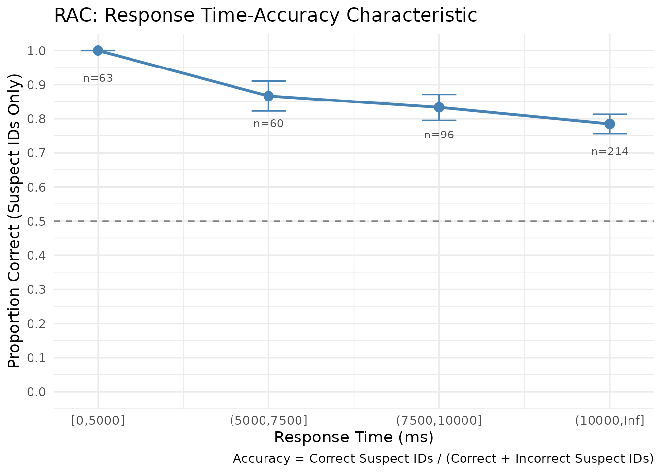

Accuracy falls as responses get slower, from about 100% in the fastest bin to about 79% in the slowest. The relationship is real but shallower than the corresponding CAC relationship, which is the usual finding: response time carries information about accuracy, but less of it than confidence does.

RAC and CAC Compared

rac <- make_rac(lineup_data, time_bins = time_bins, show_plot = FALSE)
cac <- make_cac(lineup_data, confidence_bins = c(0, 60, 80, 100),
                show_plot = FALSE)

rac$plot + ggtitle("RAC: response time and accuracy") +
  theme_minimal(base_size = 12)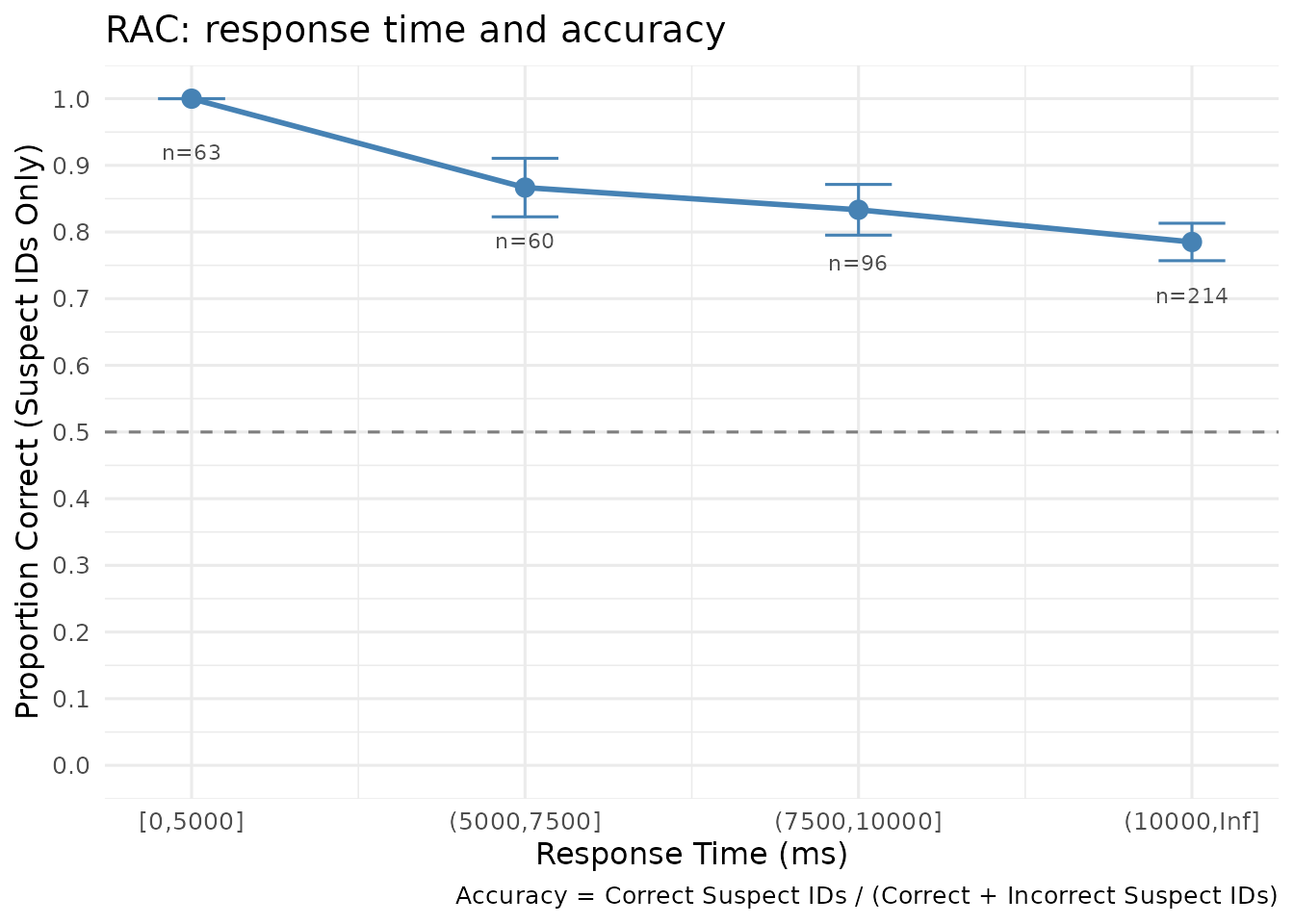

cac$plot + ggtitle("CAC: confidence and accuracy") +
  theme_minimal(base_size = 12)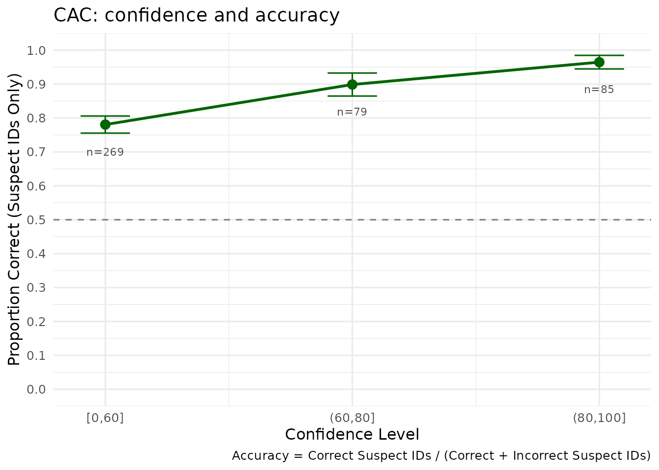

Feature	RAC	CAC
X-axis	Response time	Confidence
Measure	Recorded automatically	Self-reported
Interpretation	Faster is taken to indicate stronger memory	Higher confidence is taken to indicate stronger memory
Robustness	A recorded decision time cannot be changed by later feedback; earlier information, procedures and timing conventions can still affect it	Can be inflated by confirming feedback
Typical strength	Weaker relationship with accuracy	Stronger relationship with accuracy

The two are related but not redundant: in these data the correlation between confidence and response time is about -0.53, which leaves a good deal of independent variation.

Fine-Grained Analysis

Finer bins reveal more structure, at the cost of stability:

fine_bins <- c(seq(0, 20000, by = 2500), Inf)

rac_fine <- make_rac(lineup_data, time_bins = fine_bins, show_plot = FALSE,
                     show_errorbars = TRUE, show_n = TRUE)

knitr::kable(
  as.data.frame(rac_fine$rac_data)[, c("response_time", "n_total", "accuracy")],
  digits = 3, row.names = FALSE,
  caption = "RAC with 2.5-second bins plus an overflow bin, simulated data. Note the small n in the extreme bins."
)

RAC with 2.5-second bins plus an overflow bin, simulated data. Note the small n in the extreme bins.
response_time	n_total	accuracy
[0,2500]	15	1.000
(2500,5000]	48	1.000
(5000,7500]	60	0.867
(7500,10000]	96	0.833
(10000,12500]	97	0.804
(12500,15000]	71	0.775
(15000,17500]	36	0.750
(17500,20000]	8	0.750
(20000,Inf]	2	1.000

The extreme bins carry few observations, and their accuracy estimates should not be read as though they were as trustworthy as the well-populated middle. Always inspect n_total.

This is the fundamental awkwardness of binning: wide bins hide the shape of the relationship, narrow bins produce estimates too noisy to interpret, and there is no setting that avoids both. The next section does away with the choice.

A continuous alternative to binning

Response time is continuous, and accuracy among suspect identifications is binary — which is exactly the situation logistic regression was designed for. Rather than cutting time into bins and computing a proportion within each, we can estimate accuracy as a smooth function of time directly.

A spline term lets the shape be determined by the data rather than assumed:

fit <- glm(correct ~ splines::ns(response_time, df = 3),
           family = binomial, data = choosers)

grid <- data.frame(
  response_time = seq(min(choosers$response_time),
                      max(choosers$response_time), length.out = 200)
)
pred <- predict(fit, newdata = grid, type = "link", se.fit = TRUE)
grid$accuracy <- plogis(pred$fit)
grid$lower    <- plogis(pred$fit - 1.96 * pred$se.fit)
grid$upper    <- plogis(pred$fit + 1.96 * pred$se.fit)

ggplot(grid, aes(x = response_time / 1000, y = accuracy)) +
  geom_ribbon(aes(ymin = lower, ymax = upper), alpha = 0.2, fill = "steelblue") +
  geom_line(linewidth = 1, colour = "steelblue") +
  geom_hline(yintercept = 0.9, linetype = "dashed", colour = "red") +
  geom_rug(data = choosers,
           aes(x = response_time / 1000, y = NULL), alpha = 0.15) +
  scale_y_continuous(limits = c(0.5, 1)) +
  labs(
    x = "Response time (seconds)",
    y = "Estimated accuracy",
    title = "Continuous RAC: accuracy as a smooth function of response time",
    subtitle = "Simulated data, 600 target-present and 600 target-absent lineups. Band = 95% CI; dashed line = 90% accuracy"
  ) +
  theme_minimal(base_size = 12)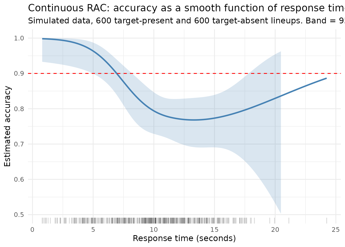

This uses every observation, requires no arbitrary boundaries, and comes with a confidence band that widens where the data thin out — visible in the rug along the bottom.

Estimating a time boundary

With a fitted curve, the question Dunning and Perretta asked can be put directly: up to what response time is estimated accuracy at least 90%?

above <- grid$response_time[grid$accuracy >= 0.90]
boundary <- if (length(above) > 0) max(above) else NA

# The fitted curve could cross 90% more than once. Count the crossings, so a
# single "boundary" is not reported when accuracy dips and recovers.
n_crossings <- sum(diff(grid$accuracy >= 0.90) != 0)

cat("Estimated accuracy at  3 s:", round(approx(grid$response_time, grid$accuracy, 3000)$y, 3), "\n")
#> Estimated accuracy at  3 s: 0.991
cat("Estimated accuracy at  8 s:", round(approx(grid$response_time, grid$accuracy, 8000)$y, 3), "\n")
#> Estimated accuracy at  8 s: 0.855
cat("Estimated accuracy at 15 s:", round(approx(grid$response_time, grid$accuracy, 15000)$y, 3), "\n\n")
#> Estimated accuracy at 15 s: 0.773
cat("Accuracy is at least 90% up to about", round(boundary / 1000, 1), "seconds\n")
#> Accuracy is at least 90% up to about 6.9 seconds
cat("Crossings of the 90% line:", n_crossings, "\n")
#> Crossings of the 90% line: 1

For these simulated data the boundary falls near 6.9 seconds. That number is a property of this dataset, and the point of Weber et al. (2004) is precisely that it will not transfer: had the simulation used a different criterion or a different d′, the boundary would move. Refitting on new data rather than importing the number is the appropriate use of the method.

Two cautions. The shaded band in the plot is a pointwise interval for accuracy at each time; it is not an interval for the boundary, which would need the whole fit bootstrapped. And a spline can cross the 90% line more than once, in which case the largest qualifying time does not mean accuracy exceeded 90% at every shorter time. The curve here crosses it once; check this before reporting a single boundary.

A note on what is being estimated. Because accuracy among suspect identifications is a positive predictive value, it depends on the proportion of target-present lineups in the design — 50% here, which is not a field base rate. The curve answers “given a suspect identification at this speed, in a study of this composition, how often is it correct?” That is the same quantity the binned RAC estimates; the continuous version simply makes it estimable without bins.

Comparing Conditions

RAC can compare experimental conditions. The comparison is only meaningful if the conditions genuinely differ, so we simulate two that do: Condition 1 has stronger memory evidence than Condition 2.

make_condition <- function(d_prime, seed) {
  d <- as.data.frame(simulate_lineup_data(
    n_tp = 400, n_ta = 400, d_prime = d_prime, c_criterion = 0.9,
    lineup_size = 6, conf_levels = 9,
    foil_bias = c(0.4, 0.2, 0.0, -0.5, -1.1), seed = seed
  ))
  d$response_time <- round(pmax(
    800, 14000 - 900 * d$confidence + rnorm(nrow(d), 0, 3500)
  ))
  d$confidence <- round(seq(20, 100, length.out = 9))[d$confidence]
  d
}

data_condition1 <- make_condition(d_prime = 2.0, seed = 201)  # good viewing
data_condition2 <- make_condition(d_prime = 1.0, seed = 202)  # poor viewing

condition1_rac <- make_rac(data_condition1, time_bins = time_bins,
                           show_plot = FALSE)
condition2_rac <- make_rac(data_condition2, time_bins = time_bins,
                           show_plot = FALSE)

comparison <- data.frame(
  `Time bin` = condition1_rac$rac_data$response_time,
  `Condition 1 (d' = 2.0)` = round(condition1_rac$rac_data$accuracy, 3),
  `Condition 2 (d' = 1.0)` = round(condition2_rac$rac_data$accuracy, 3),
  check.names = FALSE
)

knitr::kable(
  comparison, row.names = FALSE,
  caption = "RAC accuracy by condition, simulated data (400 target-present and 400 target-absent lineups per condition)."
)

RAC accuracy by condition, simulated data (400 target-present and 400 target-absent lineups per condition).
Time bin	Condition 1 (d’ = 2.0)	Condition 2 (d’ = 1.0)
[0,5000]	0.966	0.923
(5000,7500]	0.926	0.708
(7500,10000]	0.914	0.721
(10000,Inf]	0.807	0.800

Condition 1 is more accurate at every response time. Note that this is a descriptive comparison: testing whether two RAC curves differ requires a bootstrap over witnesses, which the package does not yet provide for RAC. The continuous model above offers a route to it, since a condition term and its interaction with the time spline can simply be added to the glm() call.

Custom Analysis

The binned data is available for plotting of your own:

rac_data <- rac_result$rac_data

ggplot(rac_data, aes(x = mean_time / 1000, y = accuracy)) +
  geom_point(aes(size = n_total), colour = "darkblue", alpha = 0.6) +
  geom_line(colour = "darkblue", alpha = 0.5) +
  theme_bw(base_size = 12) +
  labs(
    x = "Mean response time (seconds)",
    y = "Accuracy",
    title = "Binned RAC, simulated data",
    size = "N suspect IDs"
  ) +
  scale_y_continuous(limits = c(0, 1)) +
  geom_hline(yintercept = 0.5, linetype = "dashed")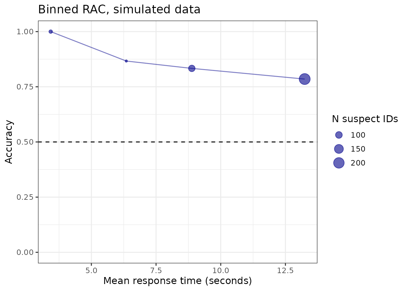

A smoother is deliberately not fitted through the four binned points here. Fitting a curve to summaries that have already discarded the within-bin variation compounds the loss rather than repairing it, and the resulting confidence band understates the uncertainty because it ignores the sample sizes behind each point. If a smooth curve is what you want, fit it to the raw observations, as in the previous section.

Technical Details

How RAC is computed

For each response time bin:

$\text{Accuracy} = \frac{\text{Correct Suspect IDs}}{\text{Correct Suspect IDs} + \text{Incorrect Suspect IDs}}$

Where:

Correct suspect IDs: target-present lineups in which the suspect was identified
Incorrect suspect IDs: target-absent lineups in which the designated innocent suspect was identified. Where no innocent suspect is designated, foil identifications divided by lineup size are used as an estimate instead

Standard errors

Standard errors assume a binomial distribution:

$SE = \sqrt{\frac{p(1-p)}{n}}$

with $p$ the accuracy and $n$ the number of suspect identifications in the bin. This treats each bin independently and takes no account of the curve being smooth, which is a further reason the continuous estimate is preferable when a shape is what interests you.

Using RAC with Real Data

Your data needs three columns, and a response time column:

my_data <- data.frame(
  target_present = c(TRUE, FALSE, TRUE, FALSE, TRUE, TRUE),
  identification = c("suspect", "filler", "suspect", "suspect",
                     "reject", "suspect"),
  response_time  = c(8234, 12456, 6789, 15020, 9310, 4870)
)

str(my_data)
#> 'data.frame':    6 obs. of  3 variables:
#>  $ target_present: logi  TRUE FALSE TRUE FALSE TRUE TRUE
#>  $ identification: chr  "suspect" "filler" "suspect" "suspect" ...
#>  $ response_time : num  8234 12456 6789 15020 9310 ...

With a dataset of adequate size you would pass it to make_rac() exactly as the simulated data was passed above. Six rows is far too few to bin, so there is no point running it here.

Points to watch:

Units. Response times must all be in the same units. The package assumes milliseconds.
Bins. Inspect the distribution first, as above. Four to six bins is common, but the number is far less important than whether each is populated.
Extreme values. Very long times often mean an interruption rather than deliberation. Consider capping rather than deleting, and report what you did.
Missing times. Trials without a recorded time are dropped, so check how many.
Sequential lineups. Response time means something different when members are viewed one at a time; total time confounds decision time with viewing time.

Exporting Results

# As CSV. Written to a temporary directory here; use your own path
outfile <- file.path(tempdir(), "rac_analysis.csv")
write.csv(rac_result$rac_data, outfile, row.names = FALSE)

knitr::kable(rac_result$rac_data, digits = 3,
             caption = "RAC analysis results, simulated data.")

RAC analysis results, simulated data.
response_time	mean_time	n_correct	n_incorrect	n_total	accuracy	se
[0,5000]	3428.746	63	0	63	1.000	0.000
(5000,7500]	6350.000	52	8	60	0.867	0.044
(7500,10000]	8882.167	80	16	96	0.833	0.038
(10000,Inf]	13244.748	168	46	214	0.785	0.028

Summary

RAC analysis puts response time on the same footing as the CAC plot puts confidence. In summary:

The idea is old (Sporer, 1993); the plot is new.
Compute it on choosers. Pooling choosers with rejections mixes two different speed-accuracy relationships and cancels most of the signal.
There is no universal time boundary. Dunning and Perretta’s 10-to-12-second rule did not replicate, and the best-separating time ranges from about 5 to 29 seconds across studies (Weber et al., 2004). Estimate it from your data.
Binning is conventional, not necessary. A logistic regression with a spline uses every observation, needs no boundaries, and gives an honest confidence band.
Response time is a weaker indicator of accuracy than confidence, and should be reported alongside it rather than instead of it.

References

Dunning, D., & Perretta, S. (2002). Automaticity and eyewitness accuracy: A 10- to 12-second rule for distinguishing accurate from inaccurate positive identifications. Journal of Applied Psychology, 87(5), 951-962.

Mickes, L. (2015). Receiver operating characteristic analysis and confidence-accuracy characteristic analysis in investigations of system variables and estimator variables that affect eyewitness memory. Journal of Applied Research in Memory and Cognition, 4(2), 93-102.

Mickes, L., Seale-Carlisle, T. M., Chen, X., & Boogert, S. (2024). pyWitness 1.0: A python eyewitness identification analysis toolkit. Behavior Research Methods, 56, 1533-1550.

Seale-Carlisle, T. M., Colloff, M. F., Flowe, H. D., Wells, W., Wixted, J. T., & Mickes, L. (2019). Confidence and response time as indicators of eyewitness identification accuracy in the lab and in the real world. Journal of Applied Research in Memory and Cognition, 8(4), 420-428.

Sporer, S. L. (1993). Eyewitness identification accuracy, confidence, and decision times in simultaneous and sequential lineups. Journal of Applied Psychology, 78(1), 22-33.

Weber, N., Brewer, N., Wells, G. L., Semmler, C., & Keast, A. (2004). Eyewitness identification accuracy and response latency: The unruly 10-12 second rule. Journal of Experimental Psychology: Applied, 10(3), 139-147.

Wixted, J. T., & Wells, G. L. (2017). The relationship between eyewitness confidence and identification accuracy: A new synthesis. Psychological Science in the Public Interest, 18(1), 10-65.

This vignette was created for r4lineups version 2.3.0

Colin G. Tredoux

Tamsyn M. Naylor

2026-11-02