Data Simulation and Power Analysis for Lineup Studies

Acknowledgement. Large language models supplied by Anthropic and OpenAI were used in preparing this vignette, to assist with checking code, testing the veracity of the approaches described, and on occasion editing the text. Responsibility for the content rests with the authors.

Introduction

Simulation is useful in lineup research for four rather different purposes, and they make different demands on the simulation.

Planning a study. How many participants are needed to detect the effect you expect? This is power analysis, and it needs a hypothesis to test.
Validating a method. If you generate data with known parameters, does your analysis recover them? This needs data whose true values you control.
Exploring designs. What happens to identification rates if the lineup has eight members instead of six? This needs only descriptive comparison.
Teaching. Showing what a criterion shift does to a lineup is easier with simulated data than with a real experiment.

library(r4lineups)

Signal Detection Theory, briefly

Signal detection theory (SDT) is the framework the simulator uses. Its assumptions are as follows.

The idea is that a witness viewing a lineup member experiences some degree of memory strength — a sense of familiarity or match to their memory of the culprit. This is treated as a continuous quantity rather than a yes/no judgement. Lineup members who are in fact the culprit tend to generate more strength than innocent members, but the distributions overlap: an unfamiliar face can occasionally feel very familiar, and a genuine culprit can occasionally feel unremarkable.

Two quantities describe this:

d′ (discriminability) is the separation between the two distributions, measured in standard deviations. It captures how good the witness’s memory is. Guilty suspects are drawn from Normal(d′, 1); foils and innocent suspects from Normal(0, 1).
The criterion is how much strength the witness requires before they are willing to identify anybody at all. It captures willingness to choose, which is a separate question from memory quality — a witness with excellent memory may still be reluctant to commit.

Keeping these separate is the central contribution of SDT to this area. Two procedures can produce identical identification rates for quite different reasons: one may improve memory, the other merely make witnesses more willing to choose. Only the first is a genuine improvement.

Decision rules

A lineup differs from a simple recognition test because the witness sees several faces and must decide among them. How the several memory strengths are combined into one decision is an open theoretical question, and the simulator implements four answers to it, following Wixted, Vul, Mickes and Wilson (2018):

Rule	The witness …
`"max"`	picks the member with the highest strength, and identifies if it clears the criterion. The independent-observations model, and the default.
`"best_rest"`	compares the best member against the average of the others, so a face only stands out if it stands out relative to the lineup.
`"ensemble"`	compares the best member against the average of the whole lineup. A rescaling of `"best_rest"`; the two are the same model with correspondingly rescaled criteria.
`"integration"`	sums strength across all members.

These are equal-variance, independent-signal versions of those models.

You are not obliged to adopt one of these models to plan a lineup study. They are how this simulator generates data, so if you use it for power analysis you are assuming one of them holds. That assumption is no different in kind from assuming a normal distribution when using a conventional power calculator. If you have pilot data, checking that the simulated identification rates resemble it is a reasonable guard against the assumption doing damage.

Attribution. The decision rules follow Wixted et al. (2018). The "max", "best_rest" and "ensemble" implementations were written with reference to the Python package pyWitness (Mickes et al., 2024), and adapted into R here; the parameter recovery in fit_winter_2ht() is checked against it. See vignette("lineup_memory_models") for the pyWitness bridge itself.

The criterion, in plainer terms

c_criterion is the strength a lineup member must reach before the witness will identify anyone. Raise it and witnesses reject more often; lower it and they choose more often.

It is important to make a point of clarification here. In textbook SDT, a criterion of 0 is “neutral”. That is not true here, because the criterion applies to the maximum of several members’ strengths, not to a single item. The maximum of six draws from Normal(0, 1) averages about 1.27, so a criterion of 0 is passed by nearly every lineup:

criteria <- c(0, 0.5, 1.0, 1.27, 1.5, 2.0)

rejection_rates <- vapply(criteria, function(cc) {
  d <- simulate_lineup_data(n_tp = 800, n_ta = 800, d_prime = 1.5,
                            c_criterion = cc, lineup_size = 6,
                            conf_levels = 5, seed = 11)
  100 * mean(d$identification[!d$target_present] == "reject")
}, numeric(1))

knitr::kable(
  data.frame(`c_criterion` = criteria,
             `TA rejection rate (%)` = round(rejection_rates, 1),
             check.names = FALSE),
  row.names = FALSE,
  caption = "Rejection rate in target-absent lineups as the criterion varies, simulated data (800 lineups of size 6 per point, d' = 1.5)."
)

Rejection rate in target-absent lineups as the criterion varies, simulated data (800 lineups of size 6 per point, d’ = 1.5).
c_criterion	TA rejection rate (%)
0.00	1.8
0.50	10.5
1.00	34.6
1.27	52.4
1.50	66.1
2.00	87.2

A criterion of 0 rejects almost nothing. The neutral value, where target-absent lineups are rejected half the time, is the median of the maximum of six standard normal draws. In a fair target-absent lineup every member’s strength is Normal(0, 1), so the maximum is below $x$ with probability $\Phi(x)^6$ , and the median is $\Phi^{-1}(0.5^{1/6}) \approx$ 1.231. The mean of the maximum, about 1.27, is close but not the same: used as the criterion it gives a rejection rate of about 52.2%.

That value therefore depends on lineup size, which is why no fixed table of “liberal / neutral / conservative” values can be given:

sizes <- c(4, 6, 8, 10, 12)

knitr::kable(
  data.frame(`Lineup size` = sizes,
             `Neutral criterion` = round(qnorm(0.5^(1 / sizes)), 3),
             check.names = FALSE),
  row.names = FALSE,
  caption = "Criterion giving 50% target-absent rejections in a fair lineup: the median of the maximum of k standard normal draws."
)

Criterion giving 50% target-absent rejections in a fair lineup: the median of the maximum of k standard normal draws.
Lineup size	Neutral criterion
4	0.998
6	1.231
8	1.385
10	1.499
12	1.588

The same formula gives any other target rejection rate $r$ : $\Phi^{-1}(r^{1/k})$ . It assumes a fair lineup with foil_bias at its default, so treat it as a starting point when foils are unequal.

A practical approach is to choose the criterion by the rejection rate it produces, rather than by its nominal value: simulate, look at the rejection rate, and adjust until it resembles the studies you are drawing on.

Basic Data Simulation

sim_data <- simulate_lineup_data(
  n_tp        = 200,   # 200 target-present lineups
  n_ta        = 200,   # 200 target-absent lineups
  d_prime     = 1.5,   # moderate discriminability
  c_criterion = 1.0,   # moderately conservative for a 6-person lineup
  lineup_size = 6,
  conf_levels = 5,
  seed        = 2026
)

head(as.data.frame(sim_data))
#>   participant_id target_present lineup_member suspect_pos identification
#> 1              4           TRUE             6           1         filler
#> 2            220          FALSE             0           1         reject
#> 3            285          FALSE             2           1         filler
#> 4            362          FALSE             3           1         filler
#> 5            298          FALSE             3           1         filler
#> 6             44           TRUE             1           1        suspect
#>   confidence
#> 1          1
#> 2          1
#> 3          3
#> 4          1
#> 5          2
#> 6          1

The output records which lineup member was chosen, not merely whether the choice happened to fall on the suspect:

lineup_member: the position chosen, with 0 for a rejection
suspect_pos: the suspect’s position
identification: "suspect", "filler" or "reject", derived from the two columns above by classify_lineup_choices()

This is important because foils are not interchangeable. By default the simulator draws every foil from the same distribution, which makes them statistically equivalent even though they are simulated separately. Real lineups are not like that: some foils are plausible alternatives to the suspect and others are barely considered. Use foil_bias to give each foil its own mean strength:

uneven <- simulate_lineup_data(
  n_tp = 400, n_ta = 400, d_prime = 1.5, c_criterion = 1.0,
  lineup_size = 6, conf_levels = 5,
  # Foil 2 is a strong alternative; foil 6 is nearly a null foil
  foil_bias = c(0.5, 0.25, 0.0, -0.4, -1.2),
  seed = 2026
)

lineup_table(uneven$lineup_member[uneven$lineup_member > 0],
             k = 6, suspect_pos = 1)
#> Lineup choices (k = 6, N = 616)
#> 
#>  pos:  1*    2   3   4   5  6
#>  cnt: 259  148  99  74  31  5
#> 
#>  * = nominated suspect

A lineup like this is unfair in a way that the collapsed "filler" label cannot express: a witness who rejects the suspect has far fewer real alternatives than the nominal size of six suggests. Simulating with foil_bias is the way to ask what that does to any measure you care about.

Power Analysis

What the function does

Power is the probability that a study of a given size detects an effect that is really there. Estimating it by simulation means: specify the effect, generate many studies of that size, run the analysis you intend to use, and count how often it reaches significance.

That last step needs a hypothesis test, which is why simulate_power_analysis() requires two conditions. d_prime is the condition of interest and d_prime_null is what it is being compared against. The default d_prime_null = 0 asks how often a study of this size could show that the procedure discriminates better than chance; setting it to a non-zero value asks the more usual question of how often two working procedures could be told apart.

Each simulated study is tested with compare_pauc(), a bootstrap comparison of partial area under the ROC curve, and power is the proportion of studies whose p-value falls below alpha.

A worked power analysis

The question: how many witnesses are needed to show that a procedure with d′ = 1.0 discriminates better than chance?

Be clear about the unit first. A sample_size of n simulates n target-present and n target-absent witnesses in each of the two conditions being compared, so 2n witnesses per condition and 4n in all; the n_total column gives the total.

# Stored with the vignette; set R4LINEUPS_PRECOMPUTE=true to recompute.
power_result <- simulate_power_analysis(
  sample_sizes  = c(25, 50, 100, 200),
  d_prime       = 1.0,
  d_prime_null  = 0,
  n_simulations = 30,   # small, so this vignette builds quickly
  n_bootstrap   = 60,   # likewise
  conf_levels   = 5,
  alpha         = 0.05,
  seed          = 2026,
  verbose       = FALSE
)

knitr::kable(
  setNames(as.data.frame(power_result)[, c("sample_size", "n_total", "power",
                                           "power_se", "mean_effect")],
           c("TP (= TA) per condition", "Total witnesses", "Power",
             "Power SE", "Mean effect")),
  digits = 3, row.names = FALSE,
  caption = "Power to detect d' = 1.0 against chance, 30 simulated studies per sample size."
)

Power to detect d’ = 1.0 against chance, 30 simulated studies per sample size.
TP (= TA) per condition	Total witnesses	Power	Power SE	Mean effect
25	100	0.367	0.088	0.033
50	200	0.733	0.081	0.026
100	400	0.833	0.068	0.026
200	800	1.000	0.000	0.032

Two things to read off. Power rises with sample size, crossing 80% between 50 and 100 target-present (and as many target-absent) witnesses per condition, that is between 200 and 400 witnesses in the whole simulated experiment. With only 30 simulations per point the crossing is itself uncertain (see the standard errors). And mean_effect — the average observed difference in pAUC — stays roughly constant across sample sizes, which is a check: sample size does not change the size of an effect, only how precisely it is measured, and sd_effect duly shrinks.

Plotting, and adjusting the plot

plot() returns an ordinary ggplot2 object, so it can be modified like any other:

p <- plot(power_result)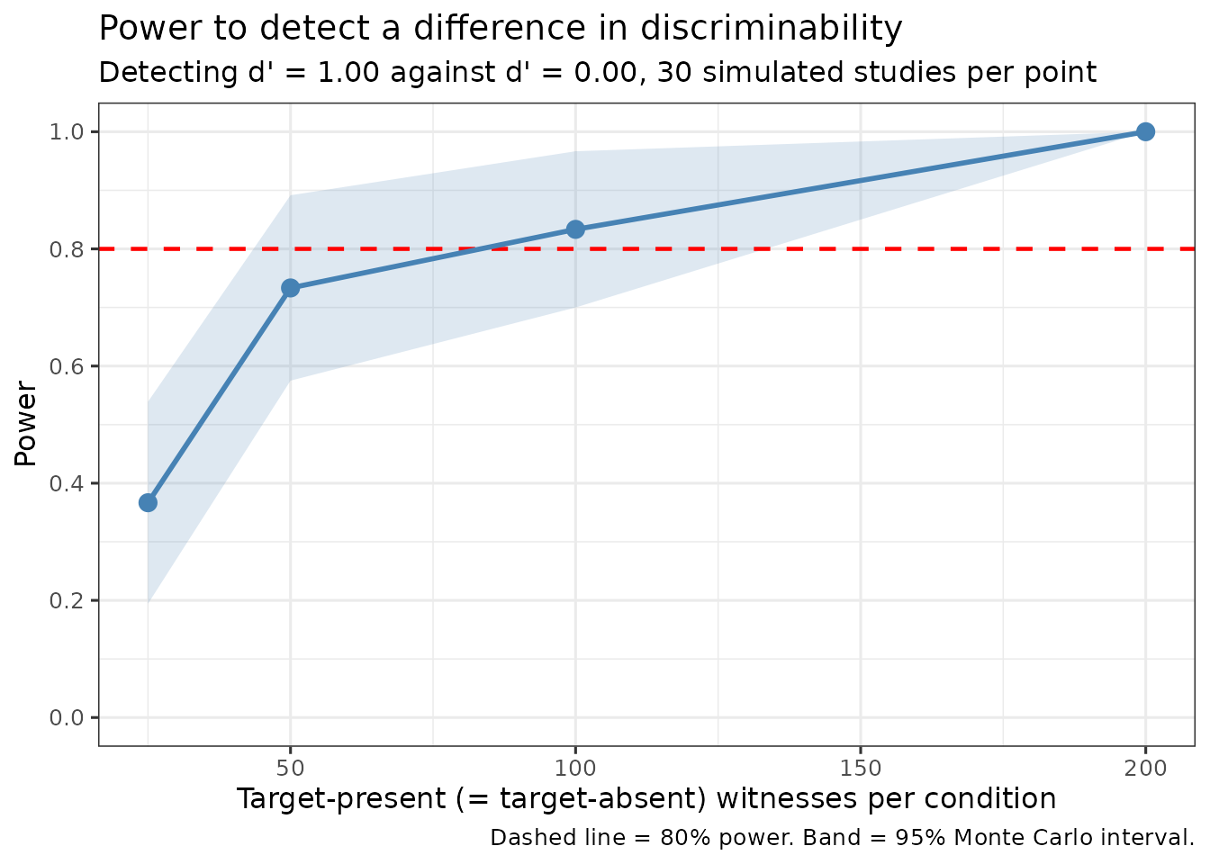

library(ggplot2)

p +
  geom_hline(yintercept = 0.95, linetype = "dotted") +
  labs(title = "Power curve with a 95% reference line") +
  theme_minimal(base_size = 12)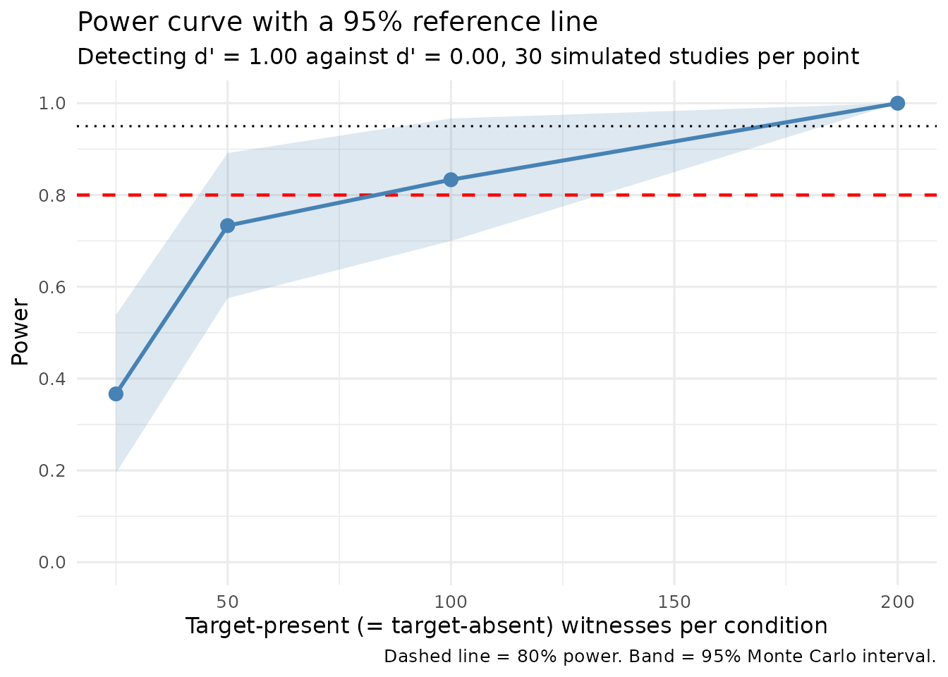

The shaded band is the Monte Carlo interval — the uncertainty in the power estimate arising from having run only 30 simulations. It is wide here, and deliberately so: with 30 simulations the standard error of an estimated power near 0.5 is about 0.09, so apparent dips between adjacent points may be nothing but noise. If a power curve looks ragged, the usual remedy is more simulations, not a different interpretation. For planning a real study, 500 to 1000 simulations per sample size is a more reasonable setting, at proportionately greater cost.

Method Check: Sensitivity to d′

A different use of simulation: generate data with a known d′, fit a model, and check that the model’s parameters move as they should. Here the 2-high-threshold model of Winter et al. is fitted to data simulated across a range of d′. The data come from a signal detection (MAX) model, so there are no true 2-HT parameter values; this checks sensitivity, not recovery.

true_dprimes <- c(0.5, 1.0, 1.5, 2.0, 2.5, 3.0)

recovery <- do.call(rbind, lapply(true_dprimes, function(dp) {
  dat <- as.data.frame(simulate_lineup_data(
    n_tp = 500, n_ta = 500, d_prime = dp, c_criterion = 1.0,
    lineup_size = 6, conf_levels = 5, seed = 321
  ))
  fit <- fit_winter_2ht(dat, lineup_size = 6,
                        target_present = "target_present",
                        identification = "identification")
  data.frame(`True d'` = dp,
             dP = round(fit$parameters[["dP"]], 3),
             dA = round(fit$parameters[["dA"]], 3),
             check.names = FALSE)
}))

knitr::kable(
  recovery, row.names = FALSE,
  caption = "2-HT detection parameters fitted to data simulated from a signal detection model at known d', 500 lineups per condition."
)

2-HT detection parameters fitted to data simulated from a signal detection model at known d’, 500 lineups per condition.
True d’	dP	dA
0.5	0.112	0.007
1.0	0.280	0.034
1.5	0.485	0.066
2.0	0.664	0.148
2.5	0.804	0.202
3.0	0.917	0.177

The detection parameter dP increases monotonically with the d′ used to generate the data, from about 0.11 to about 0.92. That shows dP is sensitive to memory strength. It does not validate the 2-HT model: dP is not on the same scale as d′, the generating model is a different model, and the exercise says nothing about bias, interval coverage or the process interpretation. Parameter recovery in the strict sense would simulate from the 2-HT equations themselves and check that the known parameters come back.

The model fits without difficulty on data of this kind. If a fit does fail, resist the temptation to wrap it in tryCatch() and report “did not converge”, because that will also swallow genuine errors such as a mis-specified column name, and you will spend a long time looking for a convergence problem that is not there.

Comparing Experimental Designs

Simulation can also answer descriptive questions about design. Here: what does lineup size do to identification rates, holding memory and willingness to choose constant?

The comparison is only interpretable if the criterion is adjusted for size. As shown earlier, a fixed criterion becomes progressively more liberal as the lineup grows, so comparing sizes at a single criterion confounds the two things we are trying to separate. We therefore set each criterion to the expected maximum for its lineup size.

sizes <- c(4, 6, 8, 10, 12)
set.seed(77)

design <- do.call(rbind, lapply(sizes, function(k) {
  # Criterion matched to lineup size, so willingness to choose is held constant
  crit <- mean(replicate(5000, max(stats::rnorm(k))))
  d <- as.data.frame(simulate_lineup_data(
    n_tp = 500, n_ta = 500, d_prime = 1.5, c_criterion = crit,
    lineup_size = k, conf_levels = 5, seed = 77
  ))
  tp <- d[d$target_present, ]; ta <- d[!d$target_present, ]
  data.frame(
    `Lineup size`          = k,
    `Criterion used`       = round(crit, 2),
    `Correct ID rate (%)`  = round(100 * mean(tp$identification == "suspect"), 1),
    `False ID rate (%)`    = round(100 * mean(ta$identification == "suspect"), 1),
    check.names = FALSE
  )
}))

knitr::kable(
  design, row.names = FALSE,
  caption = "Identification rates by lineup size at a size-matched criterion, simulated data (500 target-present and 500 target-absent lineups per size, d' = 1.5)."
)

Identification rates by lineup size at a size-matched criterion, simulated data (500 target-present and 500 target-absent lineups per size, d’ = 1.5).
Lineup size	Criterion used	Correct ID rate (%)	False ID rate (%)
4	1.04	61.2	9.8
6	1.25	49.2	9.2
8	1.42	47.6	6.8
10	1.55	39.8	3.0
12	1.63	38.2	4.2

The false identification rate falls as the lineup grows, which is the protective effect a larger lineup is meant to provide: an innocent suspect is one of more alternatives, so mistaken choices are spread more thinly. The correct identification rate is far more stable, since it depends on the culprit standing out rather than on how many foils surround them. This is the trade-off that motivates the differing lineup sizes used in practice — six is common in North American research, while police forces in the United Kingdom typically use nine foils plus the suspect, and some jurisdictions use twelve members or more.

Note that this simulation assumes every foil is equally plausible. Adding foil_bias would show the protection eroding, because a lineup of twelve in which eight are never chosen offers the protection of a much smaller one. That is the effective-size problem, and it is treated in the main vignette.

Integration with r4lineups Analyses

Simulated data works with the analysis functions directly. Running them on data whose true parameters you know is also the cheapest way to check that an analysis behaves as you expect before you point it at real data.

sim_roc <- simulate_lineup_data(
  n_tp = 300, n_ta = 300, d_prime = 1.8,
  c_criterion = 1.0, conf_levels = 5, seed = 5
)

ROC Analysis

roc_result <- make_roc(sim_roc, lineup_size = 6, show_plot = FALSE)
print(roc_result)
#> 
#> === Lineup ROC Analysis ===
#> 
#> Partial AUC: 0.056 
#> Target-present trials (N): 300 
#> Target-absent trials (N): 300 
#> Lineup size: 6 
#> Confidence levels: 5 
#> 
#> ROC Data:
#> # A tibble: 6 × 5
#>   confidence correct_id_rate false_id_rate n_correct_ids n_false_ids
#>        <dbl>           <dbl>         <dbl>         <dbl>       <dbl>
#> 1          6           0           0                   0           0
#> 2          5           0.13        0                  39           0
#> 3          4           0.243       0.00333            73           1
#> 4          3           0.437       0.02              131           6
#> 5          2           0.587       0.06              176          18
#> 6          1           0.673       0.107             202          32
#> 
#> Plot: use plot(x), or save the object and extract x$plot

make_roc() returns an object with a plot() method, which yields a ggplot object you can extend like any other:

plot(roc_result) +
  labs(title = "ROC from simulated data (d' = 1.8, 300 lineups per condition)") +
  theme_minimal(base_size = 12)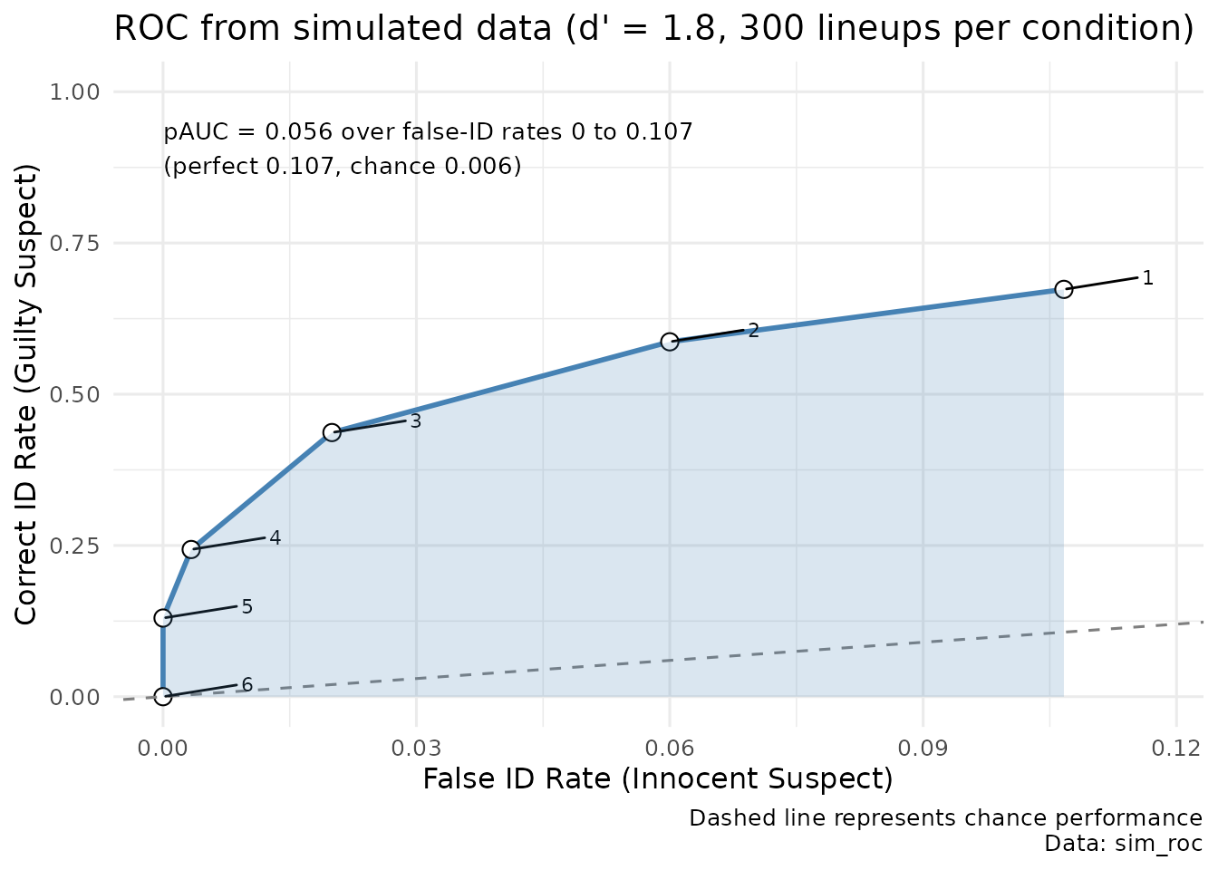

CAC Analysis

The confidence-accuracy characteristic plots accuracy against confidence, for suspect identifications only.

cac_result <- make_cac(sim_roc, show_plot = FALSE)
print(cac_result)
#> 
#> === Lineup CAC Analysis ===
#> 
#> Overall Accuracy: 0.863 
#> Total Suspect IDs: 234 
#> Lineup size: 6 
#> 
#> CAC Data:
#> # A tibble: 5 × 6
#>   confidence n_correct n_incorrect n_total accuracy     se
#>   <chr>          <int>       <int>   <int>    <dbl>  <dbl>
#> 1 1                 26          14      40    0.65  0.0754
#> 2 2                 45          12      57    0.789 0.0540
#> 3 3                 58           5      63    0.921 0.0341
#> 4 4                 34           1      35    0.971 0.0282
#> 5 5                 39           0      39    1     0     
#> 
#> Plot: use plot(x), or save the object and extract x$plot

plot(cac_result) +
  labs(title = "CAC from simulated data (d' = 1.8)") +
  theme_minimal(base_size = 12)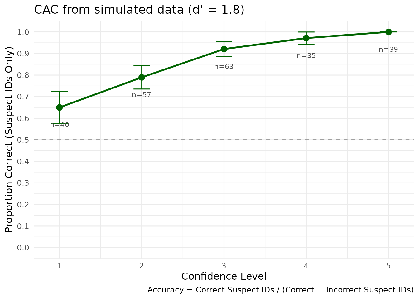

Accuracy rises across the confidence bins, from about 65% at the lowest to 100% at the highest. It should: the data were generated by a model in which confidence is a monotone function of memory strength, and memory strength is what drives accuracy. Confirming that the CAC recovers the relationship the simulator put in is a useful check that both are behaving.

RAC Analysis

The response-time analogue requires include_response_time = TRUE, which generates times from a simple model in which stronger evidence yields faster responses, with substantial noise added.

sim_rac <- simulate_lineup_data(
  n_tp = 1000, n_ta = 1000, d_prime = 1.5, c_criterion = 1.0,
  conf_levels = 5, include_response_time = TRUE, seed = 6
)

# Bins must match the data. These simulated times run from roughly 2.5 to 9.5
# seconds, so bins extending to 20 seconds would leave the upper ones empty.
round(quantile(sim_rac$response_time, c(0, 0.25, 0.5, 0.75, 1), na.rm = TRUE))
#>    0%   25%   50%   75%  100% 
#>  1628  5279  6100  6906 11167

rac_result <- make_rac(sim_rac, time_bins = c(0, 4500, 5500, 6500, Inf),
                       show_plot = FALSE)
print(rac_result)
#> 
#> === Lineup RAC Analysis ===
#> 
#> Overall Accuracy: 0.832 
#> Total Suspect IDs: 710 
#> Lineup size: 6 
#> 
#> RAC Data:
#> # A tibble: 4 × 7
#>   response_time mean_time n_correct n_incorrect n_total accuracy     se
#>   <chr>             <dbl>     <int>       <int>   <int>    <dbl>  <dbl>
#> 1 [0,4500]          3957.        82           9      91    0.901 0.0313
#> 2 (4500,5500]       5032.       177          38     215    0.823 0.0260
#> 3 (5500,6500]       5961.       185          43     228    0.811 0.0259
#> 4 (6500,Inf]        7131.       147          29     176    0.835 0.0280
#> 
#> Plot: save this object first, then extract it with x$plot

The fastest responders are the most accurate, at about 90% against roughly 82% for everyone else, after which the relationship flattens. That is a weaker and less orderly pattern than the CAC above, because the simulator’s response-time model is deliberately simple, and the noise it adds is of comparable size to the systematic component. Do not read this as evidence about response times in real witnesses — it demonstrates the mechanics of the analysis, not a substantive finding.

Choosing bins is the part that needs care. Bins fixed in advance without reference to the data will often be empty at one end, and an accuracy estimated from one or two observations will dominate the plot while meaning nothing. Inspecting the quantiles first, as above, is the simplest guard.

Full ROC Analysis

Where make_roc() uses suspect identifications, make_fullroc() uses every response, including foil identifications and rejections.

fullroc_result <- make_fullroc(sim_roc, lineup_size = 6, show_plot = FALSE)
print(fullroc_result)
#> 
#> === Full Lineup ROC Analysis (Smith & Yang, 2020) ===
#> 
#> Full AUC: 0.83 
#> Target-present trials (N): 300 
#> Target-absent trials (N): 300 
#> Lineup size: 6 
#> Ordering method: diagnosticity 
#> Operating points: 11 
#> 
#> ROC Data (first 10 points):
#>    cumulative_hit_rate cumulative_false_alarm_rate evidence_label
#> 1            0.0000000                 0.000000000         origin
#> 2            0.1300000                 0.000000000      suspect_5
#> 3            0.2433333                 0.003333333      suspect_4
#> 4            0.4366667                 0.020000000      suspect_3
#> 5            0.5866667                 0.060000000      suspect_2
#> 6            0.6733333                 0.106666667      suspect_1
#> 7            0.7500000                 0.200000000       filler_3
#> 8            0.7633333                 0.223333333       filler_4
#> 9            0.8233333                 0.396666667       filler_2
#> 10           0.9033333                 0.646666667       filler_1
#> 
#> 
#> Diagnosticity Table (ordered by evidence strength):
#>  evidence_label   hit_rate false_alarm_rate diagnosticity_ratio
#>       suspect_5 0.13000000      0.000000000         130.0000000
#>       suspect_4 0.11333333      0.003333333          34.0000000
#>       suspect_3 0.19333333      0.016666667          11.6000000
#>       suspect_2 0.15000000      0.040000000           3.7500000
#>       suspect_1 0.08666667      0.046666667           1.8571429
#>        filler_3 0.07666667      0.093333333           0.8214286
#>        filler_4 0.01333333      0.023333333           0.5714286
#>        filler_2 0.06000000      0.173333333           0.3461538
#>        filler_1 0.08000000      0.250000000           0.3200000
#>        reject_1 0.09666667      0.350000000           0.2761905
#>        filler_5 0.00000000      0.003333333           0.0000000
#> 
#> Plot: use plot(x), or save the object and extract x$plot

Because it uses the whole response distribution rather than a truncated region, the full ROC extends across the entire false-identification range and yields an ordinary AUC rather than a partial one. See vignette("fullroc_analysis") for the argument behind it.

Choosing Parameter Values

These are starting points rather than rules; revisit them against whatever literature is closest to your own design.

Discriminability (d′). Values around 1.0 are weak, 1.5 moderate, and 2.0 to 2.5 strong. Values above 3.0 are rarely observed in eyewitness studies, and a simulation resting on one will produce optimistic sample size estimates. If in doubt, plan for the smaller effect: a study powered for d′ = 1.0 will comfortably detect d′ = 2.0, whereas the reverse is not true.

Criterion. Do not choose this by its nominal value. Choose it by the rejection rate it produces, as described earlier, and remember the neutral point scales with lineup size.

Lineup size. Six is the most common in North American research; UK practice uses nine foils with the suspect, and some jurisdictions use twelve or more. Use whatever matches the procedure you are studying.

Number of simulations. The Monte Carlo standard error of an estimated power is at most sqrt(0.25 / n_simulations), which is about 0.05 at 100 simulations and 0.016 at 1000. Choose based on how precisely you need to locate the sample size, not by convention.

Seeds. Set one, and report it. Every simulation in this vignette is seeded, which is why it produces identical output each time it is built.

Summary

Key functions:

simulate_lineup_data(): generate lineup data, with foil_bias for foils that are not interchangeable
simulate_power_analysis(): power to detect a difference in discriminability
classify_lineup_choices(): derive identification outcomes from raw choices

In summary:

Power analysis needs a hypothesis test, and therefore two conditions.
The criterion is a threshold on the maximum of several strengths, so its neutral value is not zero and depends on lineup size.
A ragged power curve usually means too few simulations, and the Monte Carlo band on the plot tells you whether that is the explanation.
Simulate foils individually if the question touches lineup fairness at all.

References

Mickes, L., Seale-Carlisle, T. M., Chen, X., & Boogert, S. (2024). pyWitness 1.0: A python eyewitness identification analysis toolkit. Behavior Research Methods, 56, 1533-1550.

Wixted, J. T., & Mickes, L. (2012). The field of eyewitness memory should abandon probative value and embrace receiver operating characteristic analysis. Perspectives on Psychological Science, 7(3), 275-278.

Wixted, J. T., Vul, E., Mickes, L., & Wilson, B. M. (2018). Models of lineup memory. Cognitive Psychology, 105, 81-114.

Colin G. Tredoux

Tamsyn M. Naylor

2026-11-02