Bayesian Inference for Lineup Measures

Acknowledgement. Large language models supplied by Anthropic and OpenAI were used in preparing this vignette, to assist with checking code, testing the veracity of the approaches described, and on occasion editing the text. Responsibility for the content rests with the authors.

Purpose

This vignette shows the Bayesian posterior summaries in r4lineups for lineup fairness and confidence-based eyewitness measures.

Use these functions when you want credible intervals or direct probability statements such as $P(E' < 4.5 \mid data)$ , $P(F < 6 \mid data)$ , or $P(DR > 1 \mid data)$ . The examples use small posterior samples so that the vignette runs quickly during package checks; increase S for final analyses.

If you have only used frequentist methods

Most readers of this package will have been trained in the frequentist tradition, so this section sets out what is different here. Nothing in what follows requires accepting a philosophical position; it is mainly about what question the interval answers.

The question you probably want to ask. Having measured a six-person lineup and obtained an effective size of 4.8, a natural question is: what is the probability that this lineup’s effective size is below 4.5, a tolerance chosen before looking at the data? (Why not “below 6” is explained below: for effective size that question has the same answer, 1, whatever the data.) A frequentist confidence interval cannot answer that. It is a statement about the procedure — that intervals constructed this way contain the true value 95% of the time — not about this lineup. The true effective size either is or is not below 4.5, and frequentist probability does not attach to it.

A Bayesian credible interval does answer it. “There is a 95% probability that E′ lies between 4.1 and 5.6, given these data” is a statement about the quantity, and it is the statement most people believe they are making when they report a confidence interval.

How that is achieved. By treating the unknown quantity as having a distribution. Three steps:

A prior describes what is believed before seeing the data. Here the priors are deliberately weak — alpha = 0.5 is the Jeffreys prior for proportions, which is close to saying “no lineup member is favoured, and I am not confident about that either”.
The data update it through the likelihood.
The result is the posterior, a full distribution for the quantity, from which any summary can be read: a median, an interval, or a direct probability such as $P(E' < 4.5)$ .

Why the functions return draws rather than formulas. Effective size is $1/\sum p_i^2$ — a nonlinear function of the choice probabilities. There is no tidy closed form for its posterior. Instead the functions sample S draws from the posterior of the probabilities and transform each draw. The resulting collection of S values is the posterior of E′, and any summary is computed from it. This is why S is important: too few draws and the summaries are noisy. Note that these are independent Monte Carlo draws, not MCMC. Monte Carlo means summarising a distribution from random draws taken from it. Markov chain Monte Carlo (MCMC) is the method used when a posterior cannot be sampled directly: it builds a chain of draws, each depending on the last, that only gradually settles into the posterior, so its draws are correlated and the chain has to be checked for convergence. Here the posteriors have standard forms and can be sampled directly, so every draw is independent and there is no chain to check (see Technical Details).

What you gain in practice, beyond the interpretation:

Bounded quantities behave properly. E′ cannot exceed lineup size and a proportion cannot be negative. Normal-theory intervals can and do run outside those bounds at small samples; a posterior on the natural scale cannot.
Direct probabilities. $P(DR > 1)$ is often exactly what a report needs, and is awkward to extract from a p-value.
Small samples degrade gracefully. With few mock witnesses the posterior becomes wide, which reflects the real uncertainty, rather than producing a narrow interval resting on an asymptotic approximation that does not hold.

What it does not give you. It is not a way of getting a decisive answer from thin data. A weak prior and a small sample give a wide posterior.

library(r4lineups)

Data Shapes

The Bayesian fairness functions use mock-witness lineup choices:

a lineup vector, where each value is the chosen lineup position; or
a lineup table, where each cell is the count for one lineup position.

The Bayesian calibration function uses the standard confidence-based data frame with target_present, identification, and confidence. The SDT comparison uses summary counts: hits, misses, false alarms, and correct rejections for two conditions.

Effective Size

esize_T_bayes() fits a Dirichlet-multinomial model to the lineup choice counts and transforms each posterior draw of the choice-probability vector to Tredoux’s effective size $E'$ .

The Dirichlet distribution is a distribution over sets of probabilities that sum to 1, here the probabilities $p_1, \ldots, p_k$ that a mock witness chooses each of the $k$ lineup members. It is the multi-category generalisation of the beta distribution, which describes a single probability. It has one parameter per member, $\alpha_i$ , which acts like a count of choices imagined before seeing the data. With mock-witness counts $n_1, \ldots, n_k$ , the posterior is again Dirichlet, with parameters $n_i + \alpha_i$ : the prior counts are simply added to the observed ones. That is why the prior has little influence once there are a few dozen real choices, and why the posterior can be sampled exactly.

data(nortje2012)

lineup_vec <- nortje2012$lineup_1
k <- max(lineup_vec, na.rm = TRUE)
lineup_tab <- table(factor(lineup_vec, levels = seq_len(k)))

# An illustrative tolerance. In a real analysis choose and justify it in
# advance; the software cannot supply one.
tolerance <- 0.75 * k

set.seed(1)
esize_post <- esize_T_bayes(
  lineup_tab,
  alpha = 0.5,
  S = 1000,
  threshold = tolerance
)

esize_post
#> Bayesian Posterior: Effective Size E' (Tredoux, 1998)
#> ------------------------------------------------
#>   k (positions): 8    N (choices): 133    S (draws): 1000
#>   Prior: Dirichlet(alpha = 0.50)
#>   Posterior mean:   5.614
#>   Posterior median: 5.624
#>   95% credible interval: [4.804, 6.355]
#>   P(E' < 6.00 | data): 0.822
#>   P(E' > 6.00 | data): 0.178

plot(esize_post)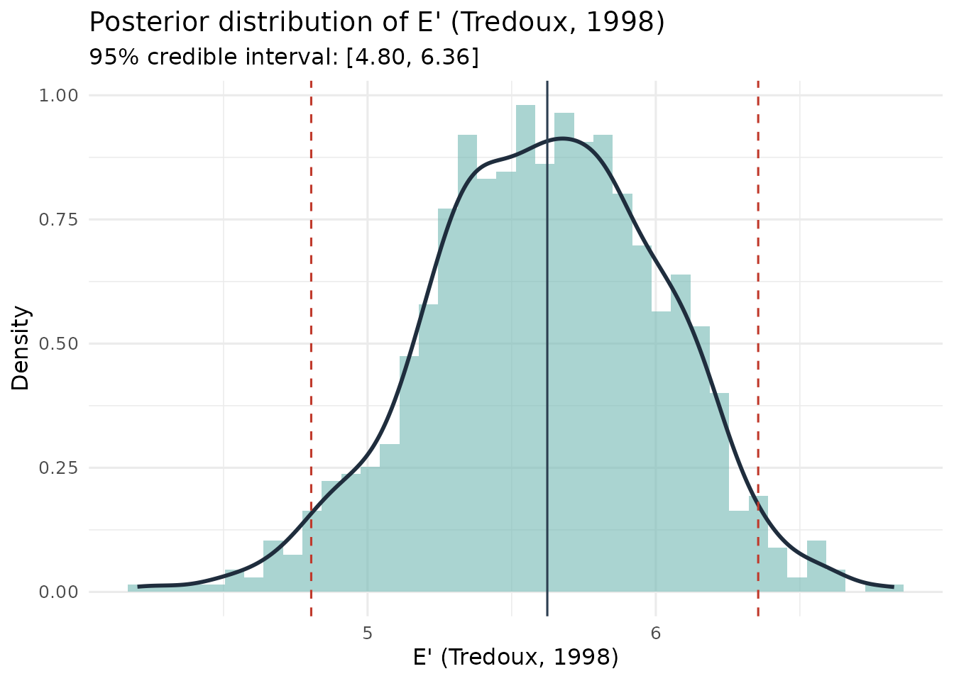

Why the threshold is not the nominal size. For any choice probabilities over $k$ members, $E' = 1/\sum p_i^2 \le k$ , with equality only when all $k$ probabilities are exactly equal. A continuous posterior gives that single point probability zero, so $P(E' < k \mid data) = 1$ for any data at all, including perfectly balanced counts; esize_T_bayes() warns if asked for it. Useful summaries are the credible interval for $E'$ , the interval for the deficit $k - E'$ , or the probability below a tolerance chosen in advance:

deficit <- k - esize_post$E_draws
knitr::kable(
  data.frame(
    Summary  = c(sprintf("95%% interval for E' (k = %d)", k),
                 "95% interval for the deficit k - E'",
                 sprintf("P(E' < %.1f | data)", tolerance)),
    Value    = c(sprintf("[%.2f, %.2f]", esize_post$credible_interval[["lower"]],
                         esize_post$credible_interval[["upper"]]),
                 sprintf("[%.2f, %.2f]", quantile(deficit, .025),
                         quantile(deficit, .975)),
                 sprintf("%.3f", esize_post$threshold_probs$P_below))
  ),
  row.names = FALSE,
  caption = "Posterior summaries of effective size, nortje2012 lineup 1."
)

Posterior summaries of effective size, nortje2012 lineup 1.
Summary	Value
95% interval for E’ (k = 8)	[4.80, 6.36]
95% interval for the deficit k - E’	[1.64, 3.20]
P(E’ < 6.0 \| data)	0.822

Functional size does not have this problem: it is not bounded above by $k$ , so $P(F < k \mid data)$ is informative.

Functional Size

func_size_bayes() models the suspect-selection rate with a beta-binomial posterior and transforms posterior draws to functional size.

set.seed(2)
func_post <- func_size_bayes(
  lineup_vec,
  target_pos = 3,
  alpha = 0.5,
  S = 1000,
  threshold = k
)

func_post
#> Bayesian Functional Size - Beta-Binomial model
#>   Prior: Jeffreys-type Beta(0.50, 0.50)
#>   n = 133, suspect IDs = 19 (rate = 0.143)
#>   Posterior mean F:   7.189
#>   Posterior median F: 6.904
#>   95% credible interval: [4.746, 10.898]
#>   P(F < 8.000 | data): 0.7480
#>   P(F > 8.000 | data): 0.2520

plot(func_post)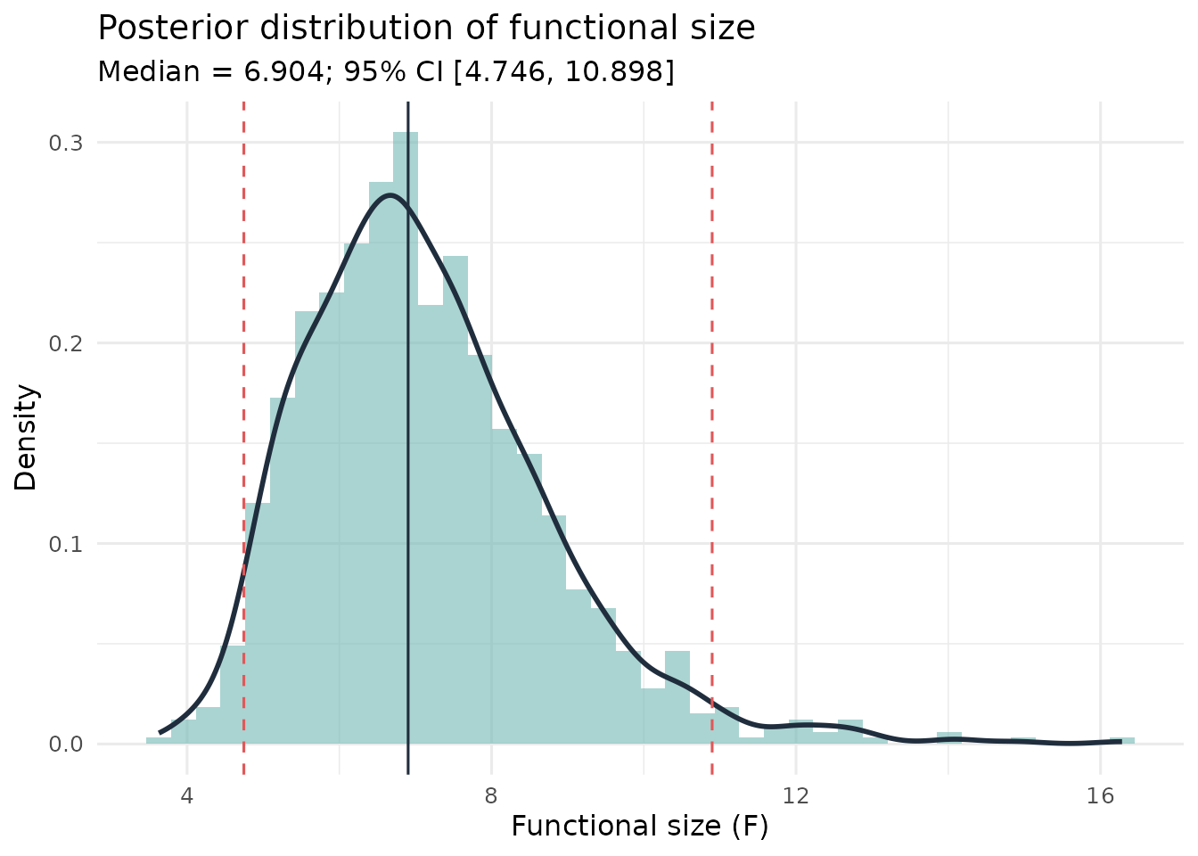

Diagnosticity Ratio

diag_ratio_T_bayes() models target-present and target-absent suspect-selection rates with independent beta-binomial posteriors and returns the posterior of the diagnosticity ratio.

tp_vec <- nortje2012$lineup_1
ta_vec <- nortje2012$lineup_2

set.seed(3)
diag_post <- diag_ratio_T_bayes(
  lineup_pres = tp_vec,
  lineup_abs = ta_vec,
  pos_pres = 3,
  pos_abs = 3,
  k1 = max(tp_vec, na.rm = TRUE),
  k2 = max(ta_vec, na.rm = TRUE),
  alpha = 0.5,
  S = 1000,
  threshold = 1
)

diag_post
#> Bayesian Diagnosticity Ratio (Tredoux) - Beta-Binomial model
#>   Prior: Jeffreys-type Beta(0.50, 0.50)
#>   TP lineup: n = 133, suspect IDs = 19
#>   TA lineup: n = 133, suspect IDs = 5
#>   Posterior mean DR:   4.301
#>   Posterior median DR: 3.645
#>   95% credible interval: [1.550, 11.214]
#>   P(DR < 1.000 | data): 0.0010
#>   P(DR > 1.000 | data): 0.9990

plot(diag_post)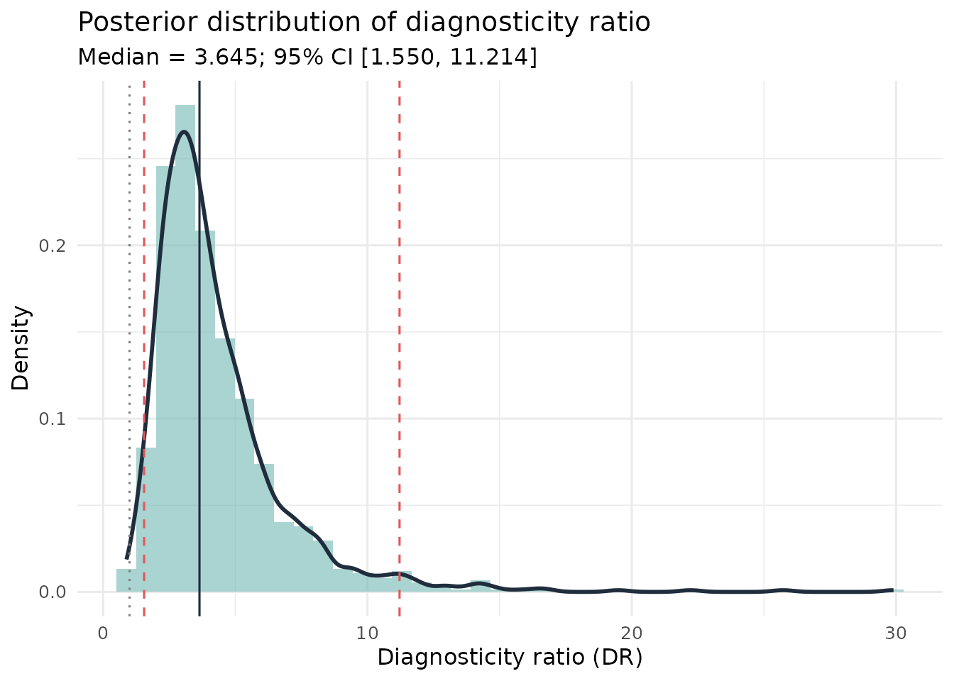

The threshold 1 is useful because $DR > 1$ indicates that suspect identifications are more common in the target-present lineup than in the target-absent lineup.

Calibration

The Bayesian calibration model conditions on bin frequencies and treats correctness within each bin as exchangeable Bernoulli observations. Fixed target-present and target-absent trial totals do not generally imply that conditional binomial likelihood. Interpret these intervals as working-model summaries for that assumption, rather than automatically exact inference for a fixed-arm experiment. Filler-derived fractional counts add another approximation; see ?calibration_bayes.

calibration_bayes() places beta posteriors on accuracy within confidence bins and propagates uncertainty into calibration $C$ , over/underconfidence $O/U$ , and normalized resolution $NRI$ .

data(lineup_example)

set.seed(4)
cal_post <- calibration_bayes(
  lineup_example,
  confidence_bins = c(0, 60, 80, 100),
  alpha = 0.5,
  S = 1000
)

cal_post
#> Bayesian Calibration Analysis - Beta-Binomial model
#>   n = 503; 3 confidence bins; prior alpha = 0.50
#>   C (calibration):      mean = 0.0729, median = 0.0727, 95% CI [0.0545, 0.0913]
#>   O/U (over/underconf): mean = -0.2268, median = -0.2266, 95% CI [-0.2564, -0.1931]
#>   NRI (resolution):     mean = 0.0450, median = 0.0447, 95% CI [0.0216, 0.0721]
#>   (Frequentist: C = 0.0727, O/U = -0.2290, NRI = 0.0453)

plot(cal_post, metric = "C")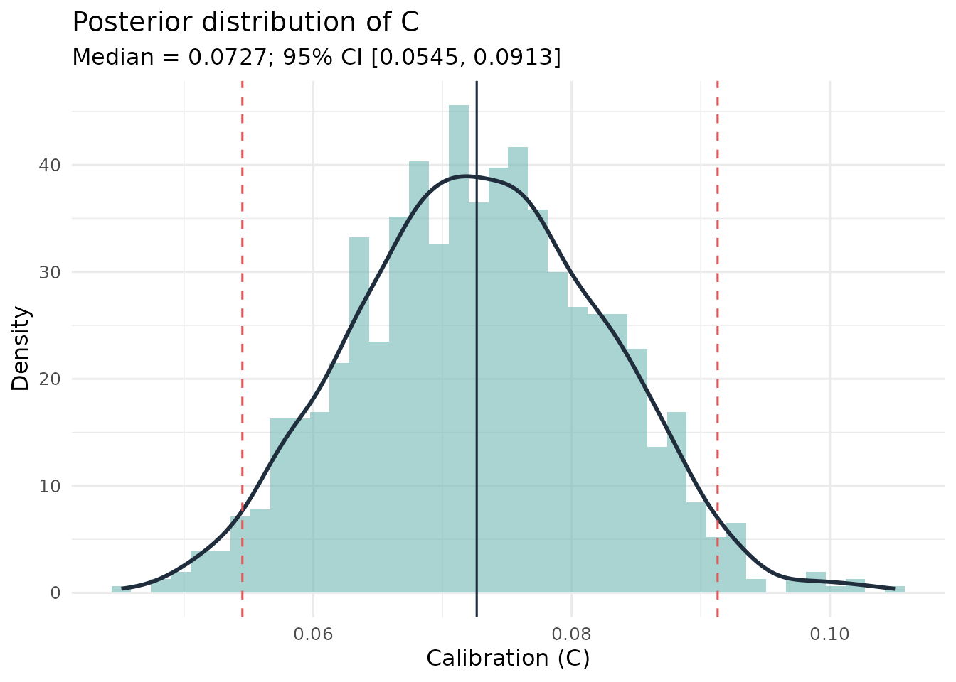

plot(cal_post, metric = "NRI")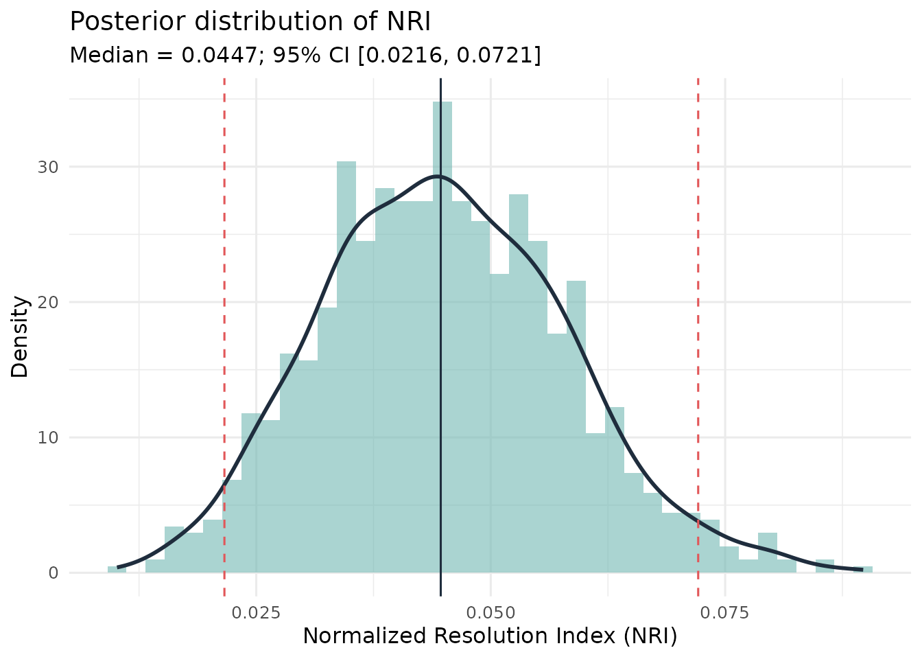

SDT d’ Comparison

sdt_compare() compares two conditions using summary SDT counts. It draws from posterior hit and false-alarm rates, converts each draw to $d'$ , and reports the posterior for $\Delta d' = d'_A - d'_B$ .

set.seed(5)
sdt_post <- sdt_compare(
  hits_A = 45, misses_A = 55, fas_A = 12, crs_A = 88,
  hits_B = 38, misses_B = 62, fas_B = 10, crs_B = 90,
  label_A = "Procedure A",
  label_B = "Procedure B",
  alpha = 0.5,
  S = 1000
)

sdt_post
#> Bayesian SDT Comparison: Procedure A vs Procedure B
#>   Prior: Jeffreys Beta(0.50, 0.50) on HR and FAR
#>   Posterior mean d': Procedure A = 1.042, Procedure B = 0.971
#>   Delta d' (Procedure A - Procedure B):
#>     Posterior mean:   0.072
#>     Posterior median: 0.072
#>     95% CI: [-0.505, 0.635]
#>   P(d'_Procedure A > d'_Procedure B | data): 0.6150
#>   P(d'_Procedure B > d'_Procedure A | data): 0.3850
#>   (Frequentist z-test: z = 0.254, p = 0.7994)

plot(sdt_post)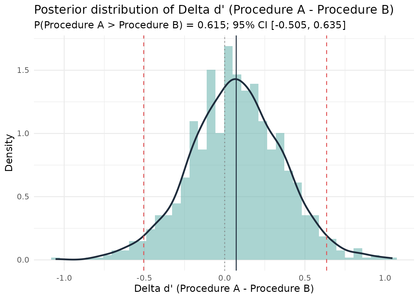

Workflow Position

These Bayesian functions complement, rather than replace, the frequentist and bootstrap functions elsewhere in the package:

use normal-theory functions for quick classical intervals where assumptions are acceptable;
use bootstrap functions when you want sampling-distribution uncertainty with minimal distributional assumptions;
use Bayesian functions when credible intervals and direct posterior probabilities are the clearest way to express uncertainty.

For substantive reports, run enough posterior draws for stable summaries and check sensitivity to the prior concentration, for example alpha = 0.1, 0.5, and 1.

sensitivity <- do.call(rbind, lapply(c(0.1, 0.5, 1.0), function(a) {
  set.seed(11)
  post <- esize_T_bayes(lineup_tab, alpha = a, S = 2000)
  data.frame(
    `Prior alpha`      = a,
    `Posterior median` = round(post$posterior_median, 3),
    `Lower`            = round(post$credible_interval[["lower"]], 3),
    `Upper`            = round(post$credible_interval[["upper"]], 3),
    check.names = FALSE
  )
}))

knitr::kable(
  sensitivity, row.names = FALSE,
  caption = "Sensitivity of the E' posterior to prior concentration, nortje2012 lineup 1 (nominal size 8)."
)

Sensitivity of the E’ posterior to prior concentration, nortje2012 lineup 1 (nominal size 8).
Prior alpha	Posterior median	Lower	Upper
0.1	5.530	4.702	6.255
0.5	5.622	4.785	6.346
1.0	5.706	4.861	6.485

If the three rows agree closely, as they generally will once there are a few dozen choices, the prior is doing little and the result is driven by the data. Disagreement is a signal that the sample is too small for the data to dominate, and should be reported rather than resolved by picking a prior.

Technical Details

What is being sampled

One definition of E′. Tredoux (1998) defined effective size through an index of diversity, $I = 1 - \sum_i p_i^2$ , transformed back to a count of members: $E' = 1/(1 - I)$ . Substituting $I$ gives $E' = 1/\sum_i p_i^2$ , the reciprocal of Simpson’s concentration index, also known as the inverse Simpson or inverse Herfindahl index. The two forms are algebraically identical; they differ only in notation, and this package uses $1/\sum_i p_i^2$ throughout. What differs between functions is the input. esize_T() substitutes the observed proportions $o_i/N$ ; esize_T_bayes() applies the same formula to each posterior draw of the true probabilities. The posterior median therefore need not equal the classical point estimate, particularly in small samples, and that gap reflects estimation, not a different definition. The bias-corrected estimate from esize_T(..., unbiased = TRUE) is a third estimator of the same quantity.

Function	Model	Transformation applied to each draw
`esize_T_bayes()`	Dirichlet-multinomial on the k choice counts	$E' = 1/\sum_i p_i^2$
`func_size_bayes()`	Beta-binomial on suspect selections	$F = 1/p_{\text{suspect}}$
`diag_ratio_T_bayes()`	Independent beta-binomials for the two lineups	$DR = p_{\text{TP}} / p_{\text{TA}}$
`calibration_bayes()`	Beta posterior on accuracy within each confidence bin	C, O/U and NRI
`sdt_compare()`	Beta posteriors on hit and false-alarm rates	$\Delta d' = d'_A - d'_B$

In each case the posterior of the transformed quantity is obtained by transforming draws, not by approximating the transformation. This is important for quantities like $DR$ , a ratio whose sampling distribution is markedly skewed: the posterior inherits that skew correctly, where a symmetric normal-theory interval would not.

The prior

alpha is the concentration parameter of the Dirichlet or beta prior, applied symmetrically. alpha = 0.5 is the Jeffreys prior, alpha = 1 is uniform, and smaller values place more weight near the boundaries. All are weak; with more than a few dozen observations the likelihood dominates, which the sensitivity check above is there to confirm.

Monte Carlo error

The posteriors here are conjugate: a Dirichlet prior with multinomial counts gives a Dirichlet posterior, and a beta prior with binomial counts gives a beta posterior. Both are standard distributions with known forms, so the functions draw from the exact posterior directly (Dirichlet draws by normalising independent gamma draws, beta draws with rbeta()). Each draw is independent of the others.

MCMC is needed only when a posterior cannot be sampled like this, typically because its normalising constant cannot be computed. A Markov chain is then constructed whose long-run distribution is the posterior; successive draws are correlated, early draws must be discarded as burn-in, and convergence has to be checked (for example with R-hat and the effective sample size). None of that applies here. $E'$ , $F$ and the other summaries are fixed transformations of each draw, so the transformed values are also independent draws from their exact posteriors, even though those posteriors have no closed form.

The practical consequences are that there is no burn-in, thinning or convergence diagnostic; the effective sample size is simply S; and Monte Carlo error falls as $1/\sqrt{S}$ . The Monte Carlo standard error of a tail probability $p$ , for example, is about $\sqrt{p(1-p)/S}$ : 0.016 for $p = 0.5$ at S = 1000, and 0.005 at S = 10000. S = 1000 is adequate for a median, but tail probabilities and interval endpoints need more; use 10,000 or more where a reported number depends on them. This simplicity rests on conjugacy: non-conjugate priors or hierarchical extensions would bring MCMC back.

Assumptions

Choices are independent across witnesses, and each witness contributes one.
The Dirichlet-multinomial prior is symmetric: every member receives the same prior count alpha, so before any choices are seen no member is expected to draw more choices than another. That is a statement of prior ignorance, not a claim that the foils are equally good in fact. The prior counts are added to the observed choices, so with even a moderate number of mock witnesses the observed differences between members dominate, and the posterior can show that a lineup is very unequal. The symmetric prior does pull small samples slightly towards equal probabilities, and so towards a larger E′, which is one reason to report the sensitivity check above.
diag_ratio_T_bayes() treats the two lineups as independent samples.
sdt_compare() assumes equal-variance signal detection, as the classical $d'$ does.

References

Tredoux, C. G. (1998). Statistical inference on measures of lineup fairness. Law and Human Behavior, 22(2), 217-237.

Colin G. Tredoux

Tamsyn M. Naylor

2026-11-02