Compare Utilities for Two Procedures

Main wrapper function to compute and plot utility comparison between two lineup procedures.

Usage

compare_utility(
  data_proc_a,
  data_proc_b,
  base_rate_grid = seq(0.01, 0.99, 0.01),
  utility_matrix = c(tp = 1, fn = -0.5, fp = -2, tn = 0.5),
  utility_type = c("max", "avg", "all"),
  show_plot = TRUE,
  innocent_suspect = "auto",
  ...
)

Arguments

data_proc_a

Dataframe for procedure A

data_proc_b

Dataframe for procedure B

base_rate_grid

Numeric vector of base rates (default: seq(0.01, 0.99, 0.01))

utility_matrix

Named vector of utilities (default: c(tp=1, fn=-0.5, fp=-2, tn=0.5))

utility_type

Character. "max", "avg", or "all" (default = "max")

show_plot

Logical. Whether to display plot (default = TRUE)

innocent_suspect

How innocent-suspect identifications in target-absent lineups are obtained. "designated": the lineups had a designated innocent suspect, so target-absent "suspect" rows are counted directly, and zero such rows means a false-ID rate of zero. "estimated": there was no designated innocent suspect, so the innocent-suspect count is estimated as filler IDs divided by lineup_size. "auto" (the default) chooses "designated" when any target-absent row is a suspect ID or the data have a non-missing suspect_pos column, and "estimated" otherwise, with a message.

...

Additional arguments passed to plot_utility_difference()

Value

A list containing difference curve data and plot

Examples

# \donttest{
data(lineup_example)
odd <- seq(1, nrow(lineup_example), by = 2)
comparison <- compare_utility(lineup_example[odd, ],
                              lineup_example[-odd, ],
                              base_rate_grid = seq(0.1, 0.9, 0.1),
                              utility_type = "max")

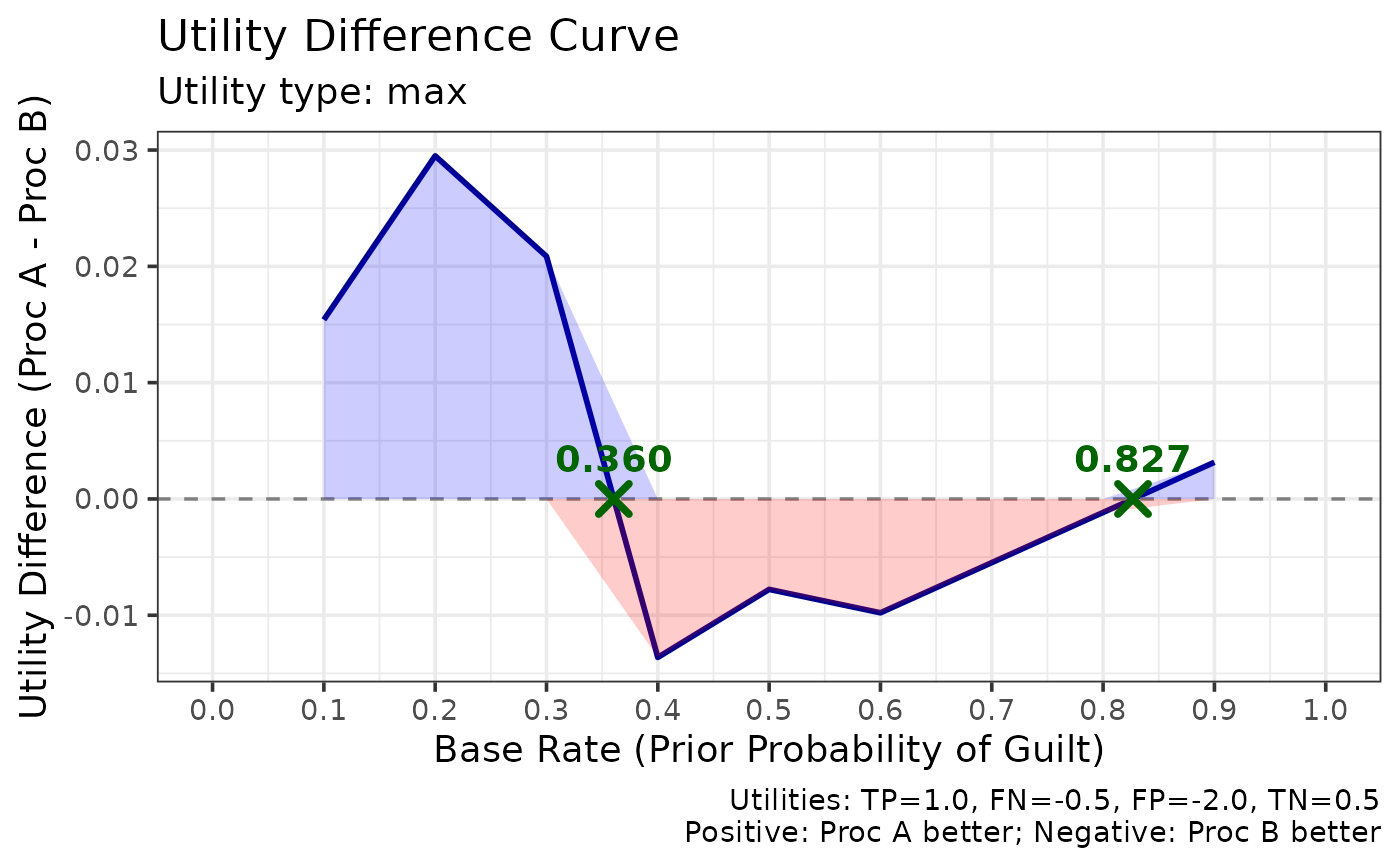print(comparison)
#> 
#> === Lineup Utility Comparison ===
#> 
#> Utility type: max 
#> Utility matrix:
#>   tp   fn   fp   tn 
#>  1.0 -0.5 -2.0  0.5 
#> 
#> Crossover points (base rates where procedures are equivalent):
#>    0.360, 0.827 
#> 
#> Utility difference at key base rates:
#>   (Positive = Proc A better; Negative = Proc B better)
#> 
#>   Base rate 0.1: +0.0154
#>   Base rate 0.3: +0.0209
#>   Base rate 0.5: -0.0078
#>   Base rate 0.7: -0.0055
#>   Base rate 0.9: +0.0032
#> 
#> Plot: save this object first, then extract it with x$plot
# }