Plot Calibration Curve

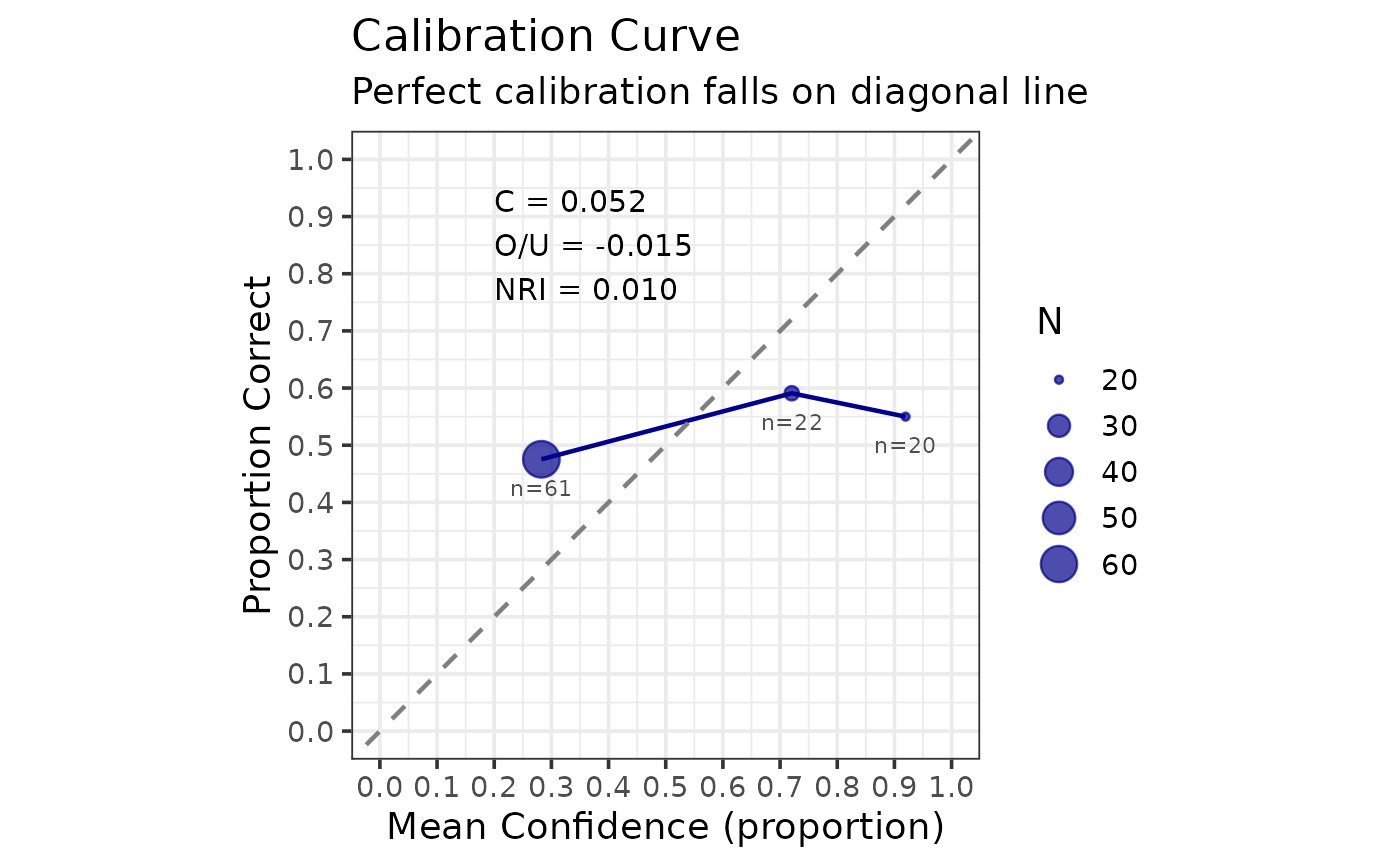
Creates a calibration curve plot showing the relationship between confidence and accuracy. A perfectly calibrated witness would fall on the diagonal line.

Usage

make_calibration_gg(
  cal_obj,
  show_stats = TRUE,
  show_n = TRUE,
  show_diagonal = TRUE
)

Arguments

cal_obj

List output from make_calibration_data()

show_stats

Logical. Whether to display calibration statistics on plot (default = TRUE)

show_n

Logical. Whether to show sample sizes per bin (default = TRUE)

show_diagonal

Logical. Whether to show perfect calibration line (default = TRUE)

Value

A ggplot2 object

Details

The calibration curve plots mean confidence (x-axis) against accuracy (y-axis) for each confidence bin. Points on the diagonal indicate perfect calibration. Points above the diagonal indicate underconfidence, while points below indicate overconfidence.

Examples

set.seed(123)
n <- 200
data <- data.frame(
  target_present = rep(c(TRUE, FALSE), each = n / 2),
  identification = sample(c("suspect", "filler", "reject"), n,
                          replace = TRUE, prob = c(0.5, 0.25, 0.25)),
  confidence = round(runif(n, 0, 100))
)
cal <- make_calibration_data(data, confidence_bins = c(0, 60, 80, 100))
make_calibration_gg(cal)