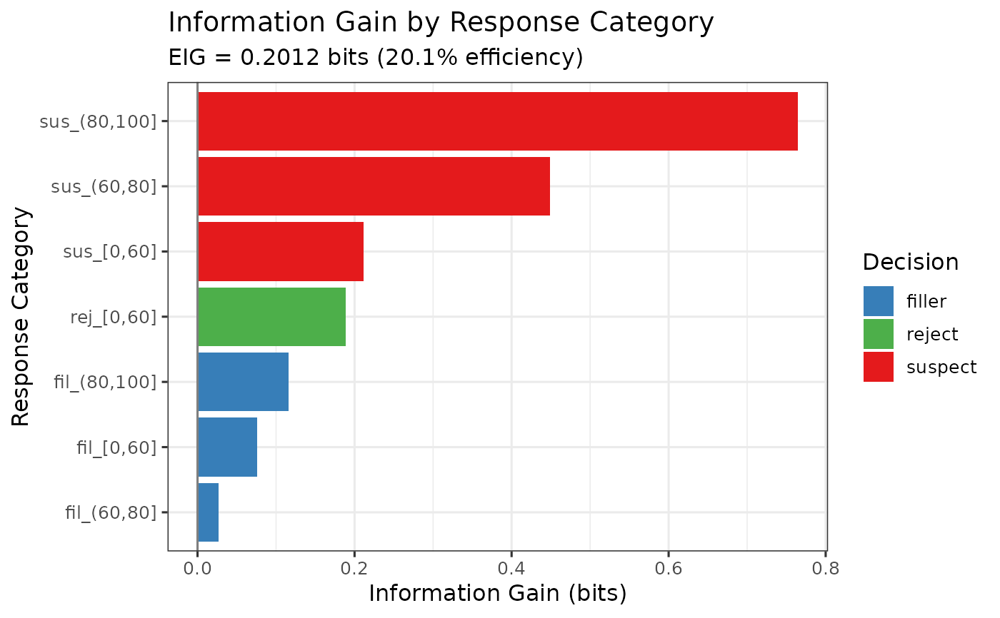
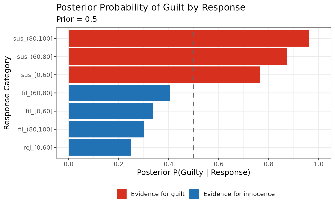
Convenience wrapper that computes EIG and creates visualizations.
Usage
make_eig(
  data,
  prior_guilt = 0.5,
  confidence_bins = NULL,
  show_plot = TRUE,
  plot_type = "both",
  lineup_size = 6,
  innocent_suspect = "auto"
)
Arguments
- data
A dataframe with columns: target_present, identification, confidence
- prior_guilt
Numeric. Prior probability that suspect is guilty (default = 0.5)
- confidence_bins
Numeric vector of bin edges (optional)
- show_plot
Logical. Whether to create plots (default = TRUE)
- plot_type
Character. Which plot to create: "ig" (information gain), "posteriors" (posterior probabilities), or "both" (default)
- lineup_size
Nominal lineup size used when no designated innocent suspect is present.
- innocent_suspect
How innocent-suspect identifications in target-absent lineups are obtained.
"designated": the lineups had a designated innocent suspect, so target-absent"suspect"rows are counted directly, and zero such rows means a false-ID rate of zero."estimated": there was no designated innocent suspect, so the innocent-suspect count is estimated as filler IDs divided bylineup_size."auto"(the default) chooses"designated"when any target-absent row is a suspect ID or the data have a non-missingsuspect_poscolumn, and"estimated"otherwise, with a message.