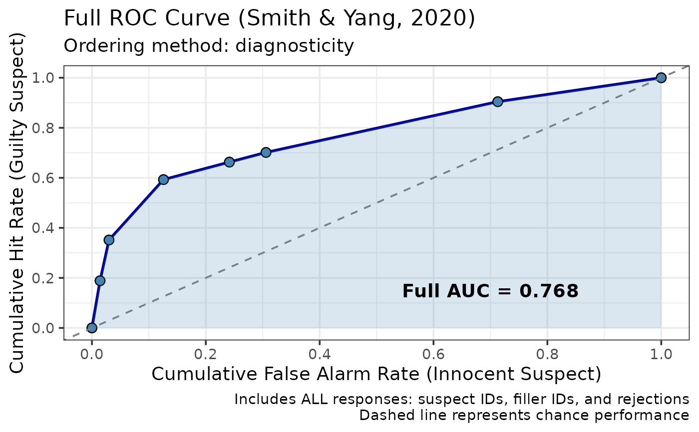
Main function to compute and plot a full ROC curve using all eyewitness responses (suspect ID, filler ID, rejection) following Smith & Yang (2020).
Usage
make_fullroc(
  data,
  conf_bins = NULL,
  order = c("diagnosticity", "apriori"),
  lineup_size = 6,
  show_plot = TRUE,
  epsilon = 0.001,
  innocent_suspect = "auto",
  ...
)
Arguments
- data
A dataframe with columns: target_present, identification, confidence
- conf_bins
Numeric vector for confidence bin boundaries (default = NULL)
- order
Character. "diagnosticity" or "apriori" (default = "diagnosticity")
- lineup_size
Integer. Number of people in lineup (default = 6)
- show_plot
Logical. Whether to display the plot (default = TRUE)
- epsilon
Numeric. Small value for FAR = 0 cases (default = 0.001)
- innocent_suspect
How innocent-suspect identifications in target-absent lineups are obtained.
"designated": the lineups had a designated innocent suspect, so target-absent"suspect"rows are counted directly, and zero such rows means a false-ID rate of zero."estimated": there was no designated innocent suspect, so the innocent-suspect count is estimated as filler IDs divided bylineup_size."auto"(the default) chooses"designated"when any target-absent row is a suspect ID or the data have a non-missingsuspect_poscolumn, and"estimated"otherwise, with a message.- ...
Additional arguments passed to plot_fullroc()
Value
A list containing:
plot: ggplot2 object. Always returned, whatever show_plot is set to; show_plot controls only whether it is displayed immediately
roc_data: Dataframe with ROC curve points
auc: Full area under the curve
diagnosticity_table: Table with diagnosticity ratios
summary: Summary statistics
Details
This is the main user-facing function for computing full ROC curves. It calls make_fullroc_data() to compute the ROC, then plot_fullroc() to visualize it.
References
Smith, A. M., Yang, Y., & Wells, G. L. (2020). Distinguishing between investigator discriminability and eyewitness discriminability: A method for creating full receiver operating characteristic curves of lineup identification performance. Perspectives on Psychological Science, 15(3), 589-607.
Examples
data(lineup_example)
# Compute and plot full ROC
result <- make_fullroc(lineup_example)
#> Ordering categories by their sample diagnosticity ratios is optimistically biased: the ordering is estimated from the same data used to compute the AUC. With roughly 700 lineups per arm the bias can be substantial. Use order = "apriori" for inference or between-condition comparisons; see vignette("fullroc_analysis").
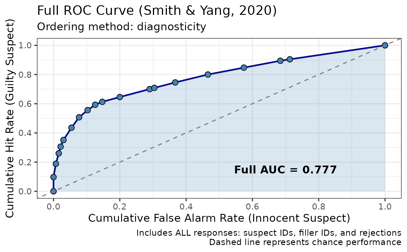 print(result$auc)
#> [1] 0.7774776
# With custom confidence bins
result2 <- make_fullroc(lineup_example, conf_bins = c(0, 60, 80, 100))
#> Ordering categories by their sample diagnosticity ratios is optimistically biased: the ordering is estimated from the same data used to compute the AUC. With roughly 700 lineups per arm the bias can be substantial. Use order = "apriori" for inference or between-condition comparisons; see vignette("fullroc_analysis").