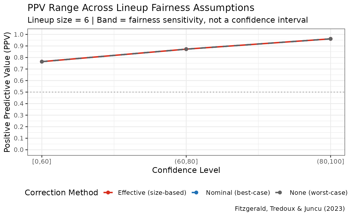
Creates a ggplot visualization showing the range of PPV estimates across the three correction methods (nominal, effective, none) as recommended by Fitzgerald et al. (2023).
Details
The plot shows three curves:
Nominal (blue, dashed): Best-case estimate assuming fair lineup
Effective (red, solid): Size-based approximation accounting for uneven choices
None (gray, dashed): Worst-case estimate (no correction)
The shaded band between nominal and none represents the PPV uncertainty range due to unknown lineup fairness conditions. The effective size estimate typically falls within this range and is a size-based approximation, not a validated best estimate.
References
Fitzgerald, R. J., Tredoux, C. G., & Juncu, S. (2023). Estimation of eyewitness error rates in fair and biased lineups. Law and Human Behavior.
Examples
data(lineup_example)
ppv_range <- ppv_range_by_confidence(lineup_example,
                                     confidence_bins = c(0, 60, 80, 100))
#> Target-absent lineups contain a designated innocent suspect, so innocent-suspect IDs are counted directly and no lineup-size correction is applied. The nominal, effective and uncorrected estimates are therefore identical for these data. The three diverge only when no innocent suspect is designated and the number of innocent-suspect IDs has to be estimated from the filler IDs.
plot_ppv_range(ppv_range)