Bayesian Calibration Analysis (Beta-Binomial Model)

Computes Bayesian posterior distributions for the calibration statistic C, over/underconfidence (O/U), and the Normalized Resolution Index (NRI) by placing independent Beta priors on the accuracy rate in each confidence bin.

Usage

calibration_bayes(
  data,
  confidence_bins = NULL,
  choosers_only = TRUE,
  lineup_size = 6,
  alpha = 0.5,
  S = 10000,
  credible_mass = 0.95,
  confidence_scale = c("auto", "0-1", "0-100"),
  innocent_suspect = "auto"
)

Arguments

data: A dataframe with columns target_present (logical), identification (character: "suspect", "filler", "reject"), and confidence (numeric).
confidence_bins: Numeric vector of bin edges for confidence (e.g., c(0, 60, 80, 100)). If NULL (default), treats each unique confidence level as its own bin.
choosers_only: Logical. If TRUE (default), only suspect identifications are included (standard eyewitness calibration practice).
lineup_size: Integer. Number of lineup members (default 6).
alpha: Prior concentration for the Beta prior on per-bin accuracy. Default 0.5 (Jeffreys). Named shortcuts: "jeffreys", "uniform", "weak".
S: Number of posterior draws per bin. Default 10000.
credible_mass: Width of equal-tailed credible intervals. Default 0.95.
confidence_scale: How the confidence scale is interpreted: "auto" (default), "0-1", or "0-100". See make_calibration_data.
innocent_suspect: How innocent-suspect identifications in target-absent lineups are obtained. "designated": the lineups had a designated innocent suspect, so target-absent "suspect" rows are counted directly, and zero such rows means a false-ID rate of zero. "estimated": there was no designated innocent suspect, so the innocent-suspect count is estimated as filler IDs divided by lineup_size. "auto" (the default) chooses "designated" when any target-absent row is a suspect ID or the data have a non-missing suspect_pos column, and "estimated" otherwise, with a message.

Value

An object of class "calibration_bayes" containing:

C_draws, OU_draws, NRI_draws: Posterior draws of each statistic.
C_mean, C_median, C_ci: Posterior mean, median, and credible interval for C.
OU_mean, OU_median, OU_ci: Same for O/U.
NRI_mean, NRI_median, NRI_ci: Same for NRI.
point_estimates: Frequentist C, OU, NRI from make_calibration_data().
bin_data: Per-bin summary (n, n_correct, mean_confidence, accuracy).
prior_alpha, S, credible_mass, n_total: Metadata.

Details

For each confidence bin $j$ with $n_j$ responses and $k_j$ correct identifications, the posterior accuracy is: $$a_j \mid \mathbf{n} \sim \mathrm{Beta}(k_j + \alpha,\; n_j - k_j + \alpha).$$ For each posterior draw $s$, the calibration statistics are computed: $$C^{(s)} = \sum_j \frac{n_j}{N}(c_j - a_j^{(s)})^2$$ $$OU^{(s)} = \bar{c} - \sum_j \frac{n_j}{N} a_j^{(s)}$$ $$NRI^{(s)} = \frac{\sum_j \frac{n_j}{N}(a_j^{(s)} - \bar{a}^{(s)})^2}{\bar{a}^{(s)}(1-\bar{a}^{(s)})}$$ where $c_j$ is the mean confidence (proportion scale) in bin $j$ and $\bar{c}$ is the overall mean confidence. This model assumes exchangeable Bernoulli correctness within each bin. In experiments with fixed TP and TA totals, conditioning on the number of identifications in a bin does not generally give a binomial correct count. These intervals are therefore conditional working-model summaries, rather than automatically exact posterior inference for that fixed-arm design. If innocent IDs are estimated from fillers, the fractional effective counts produce a working Beta posterior, not the exact likelihood for observed designated-suspect counts. Its intervals do not propagate all uncertainty in that estimation. Bin frequencies and mean confidence are conditioned on.

References

Juslin, P., Olsson, N., & Winman, A. (1996). Calibration and diagnosticity of confidence in eyewitness identification. Journal of Experimental Psychology: Learning, Memory, and Cognition, 22(5), 1304-1316.

Brewer, N., & Wells, G. L. (2006). The confidence-accuracy relationship in eyewitness identification. Journal of Experimental Psychology: Applied, 12(1), 11-30.

Examples

set.seed(42)
n <- 200
conf  <- sample(c(50, 70, 90), n, replace = TRUE)
tp    <- sample(c(TRUE, FALSE), n, replace = TRUE)
ident <- ifelse(tp, "suspect", sample(c("suspect","filler","reject"), n, replace=TRUE))
df    <- data.frame(target_present = tp, identification = ident, confidence = conf)
res   <- calibration_bayes(df, confidence_bins = c(0, 60, 80, 100))
print(res)
#> Bayesian Calibration Analysis - Beta-Binomial model
#>   n = 131; 3 confidence bins; prior alpha = 0.50
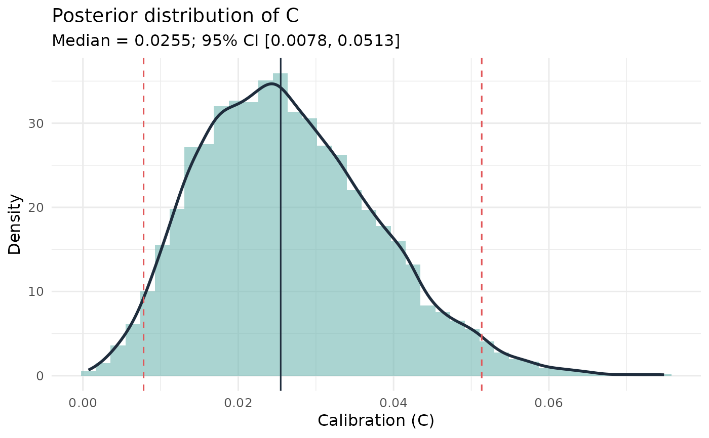
#>   C (calibration):      mean = 0.0266, median = 0.0255, 95% CI [0.0078, 0.0513]
#>   O/U (over/underconf): mean = -0.1147, median = -0.1159, 95% CI [-0.1792, -0.0420]
#>   NRI (resolution):     mean = 0.0327, median = 0.0274, 95% CI [0.0014, 0.0947]
#>   (Frequentist: C = 0.0239, O/U = -0.1214, NRI = 0.0219)
plot(res)