Bayesian Posterior Distribution of Effective Size (Tredoux, 1998)

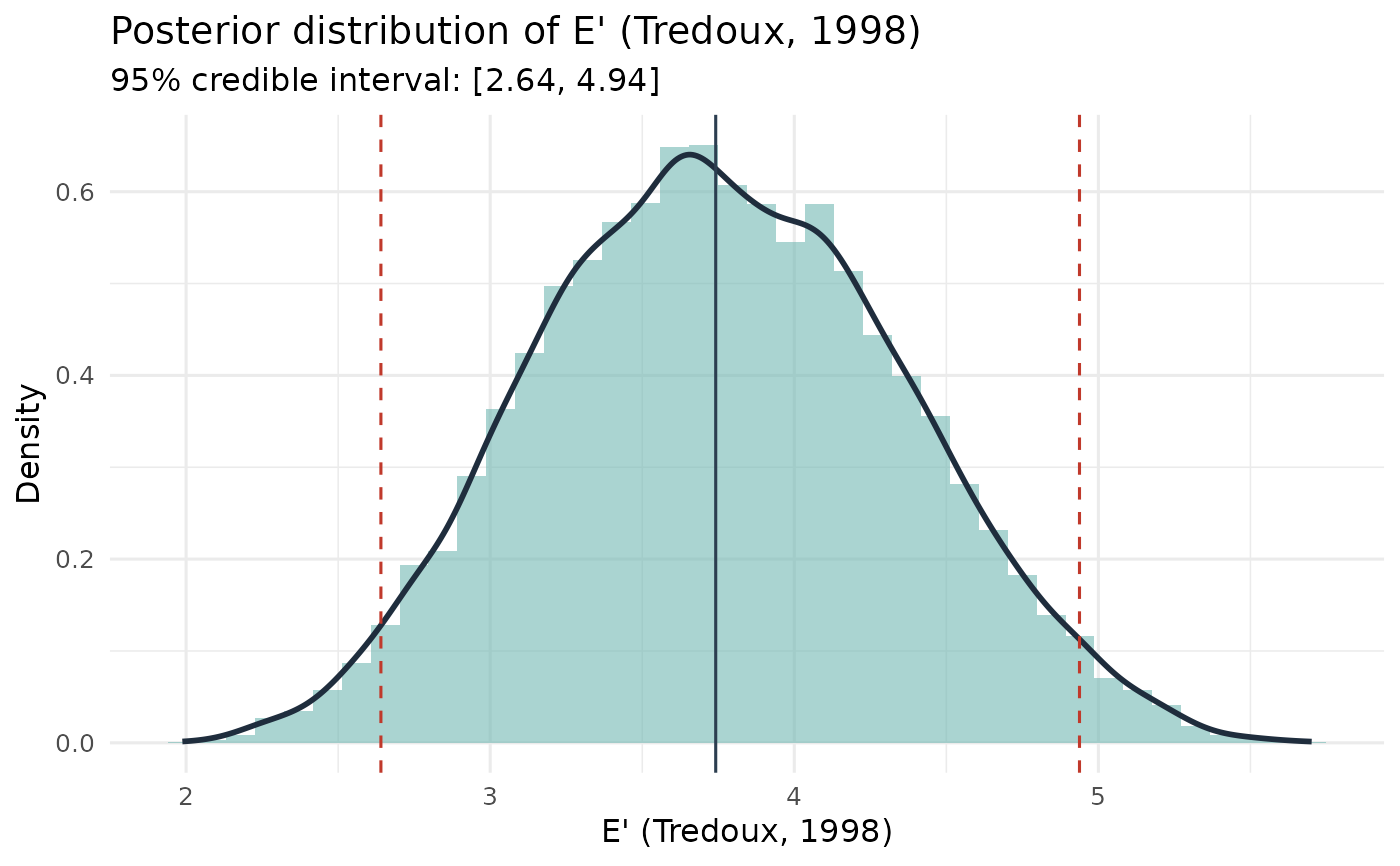
Fits a Dirichlet-Multinomial conjugate model to mock-witness choice counts and returns the posterior distribution of effective size E' (Tredoux, 1998).

Usage

esize_T_bayes(
  lineup_tab,
  alpha = 0.5,
  S = 10000,
  credible_mass = 0.95,
  threshold = NULL
)

Arguments

lineup_tab: A table of lineup choice counts (one entry per position).
alpha: Dirichlet concentration parameter(s). A scalar (applied to all k positions) or a length-k numeric vector. Typical choices: 0.5 (Jeffreys prior, default), 1 (uniform over the simplex), 0.1 (weakly informative). Smaller values allow the posterior to concentrate more sharply around the observed proportions.
S: Number of posterior draws. Default 10000.
credible_mass: Width of the equal-tailed credible interval. Default 0.95.
threshold: Optional finite scalar. When supplied, the function also reports P(E' < threshold | data) and P(E' > threshold | data), enabling direct probability statements about whether the lineup is functioning below or above a fairness benchmark. Because E' <= k for every choice-probability vector, with equality only when all k probabilities are exactly equal, P(E' < k | data) is 1 under any continuous posterior, however uniform the data. A threshold of k or more therefore carries no information, and the function warns. Use a tolerance below k that you choose and justify in advance (for example 0.8 k), or report the credible interval for E' or for the deficit k - E'.

Value

An object of class "esize_T_bayes" containing:

E_draws: Numeric vector of S posterior draws of E'.
posterior_mean: Posterior mean of E'.
posterior_median: Posterior median of E'.
credible_interval: Named 2-vector (lower, upper) giving the equal-tailed credible interval.
prior_alpha: The alpha vector used.
n: Total number of mock-witness choices.
k: Number of lineup positions.
S: Number of posterior draws.
credible_mass: Credible interval width.
threshold: Threshold value supplied, or NULL.
threshold_probs: List with P_below and P_above, or NULL when no threshold was supplied.

Details

Effective size E' = 1/sum(p_i^2) (Tredoux, 1998) is mathematically identical to the reciprocal of the Herfindahl-Hirschman concentration index (Herfindahl, 1950; Hirschman, 1945) and to the reciprocal of Simpson's (1949) concentration statistic lambda. The Bayesian approach estimates the latent choice-probability vector p rather than E' directly.

With mock-witness counts n = (n_1, ..., n_k) and a Dirichlet prior: $$p \sim \mathrm{Dirichlet}(\alpha_1, \ldots, \alpha_k),$$ the posterior is conjugate: $$p \mid n \sim \mathrm{Dirichlet}(n_1 + \alpha_1, \ldots, n_k + \alpha_k).$$ Each posterior draw of p is mapped to a draw of E' via E'(p) = 1/sum(p_i^2). The resulting posterior distribution of E' summarises uncertainty about effective lineup size given the observed choices.

Dirichlet samples are generated by normalising independent Gamma draws (base R only; no additional package dependencies).

For publication, a prior sensitivity analysis using at least alpha = 0.5, 1, and 0.1 is recommended. If the substantive conclusion changes across these priors, the mock-witness sample is likely too small to support a confident fairness conclusion.

References

Herfindahl, O. C. (1950). Concentration in the US steel industry. Doctoral dissertation, Columbia University.

Hirschman, A. O. (1945). National power and the structure of foreign trade. University of California Press.

Simpson, E. H. (1949). Measurement of diversity. Nature, 163, 688.

Tredoux, C. G. (1998). Statistical inference on measures of lineup fairness. Law and Human Behavior, 22(2), 217-237.

Examples

counts <- c(18, 7, 5, 4, 3, 3)
lineup_tab <- as.table(setNames(counts, 1:6))

# Default Jeffreys prior
result <- esize_T_bayes(lineup_tab)
print(result)
#> Bayesian Posterior: Effective Size E' (Tredoux, 1998)
#> ------------------------------------------------
#>   k (positions): 6    N (choices): 40    S (draws): 10000
#>   Prior: Dirichlet(alpha = 0.50)
#>   Posterior mean:   3.757
#>   Posterior median: 3.742
#>   95% credible interval: [2.641, 4.938]

# With a fairness threshold
result2 <- esize_T_bayes(lineup_tab, threshold = 4)
print(result2)
#> Bayesian Posterior: Effective Size E' (Tredoux, 1998)
#> ------------------------------------------------
#>   k (positions): 6    N (choices): 40    S (draws): 10000
#>   Prior: Dirichlet(alpha = 0.50)
#>   Posterior mean:   3.767
#>   Posterior median: 3.764
#>   95% credible interval: [2.647, 4.952]
#>   P(E' < 4.00 | data): 0.653
#>   P(E' > 4.00 | data): 0.347

# Plot the posterior
plot(result)