Bayesian Diagnosticity Ratio (Tredoux, Beta-Binomial Model)

Computes a Bayesian posterior distribution for the Tredoux diagnosticity ratio using independent Beta-Binomial models for the target-present and target-absent suspect-selection rates.

Usage

diag_ratio_T_bayes(
  lineup_pres,
  lineup_abs,
  pos_pres,
  pos_abs,
  k1,
  k2,
  alpha = 0.5,
  S = 10000,
  credible_mass = 0.95,
  threshold = NULL
)

Arguments

lineup_pres: A numeric vector of lineup choices for a target-present lineup.
lineup_abs: A numeric vector of lineup choices for a target-absent lineup.
pos_pres: Scalar; suspect position in the target-present lineup.
pos_abs: Scalar; suspect position in the target-absent lineup.
k1: Number of members in the target-present lineup (for input validation).
k2: Number of members in the target-absent lineup (for input validation).
alpha: Dirichlet concentration (prior strength). A scalar $\alpha > 0$ applied to both cells. Named shortcuts: "jeffreys" (0.5, default), "uniform" (1), "weak" (0.1).
S: Number of posterior draws. Default 10000.
credible_mass: Width of the equal-tailed credible interval. Default 0.95.
threshold: Optional numeric. If supplied, reports $P(DR < t)$ and $P(DR > t | \mathbf{n})$.

Value

An object of class "diag_ratio_T_bayes" containing:

DR_draws: Numeric vector of length S: posterior draws of DR.
lnDR_draws: Log-transformed posterior draws.
posterior_mean, posterior_median: Posterior point estimates. The mean is exact, and is Inf when it does not exist (see Details).
credible_interval: Named two-element vector (lower, upper).
prior_alpha: Alpha value used.
n_tp, n_ta, S, credible_mass: Input metadata.
threshold, threshold_probs: Threshold and associated probabilities (or NULL).

Details

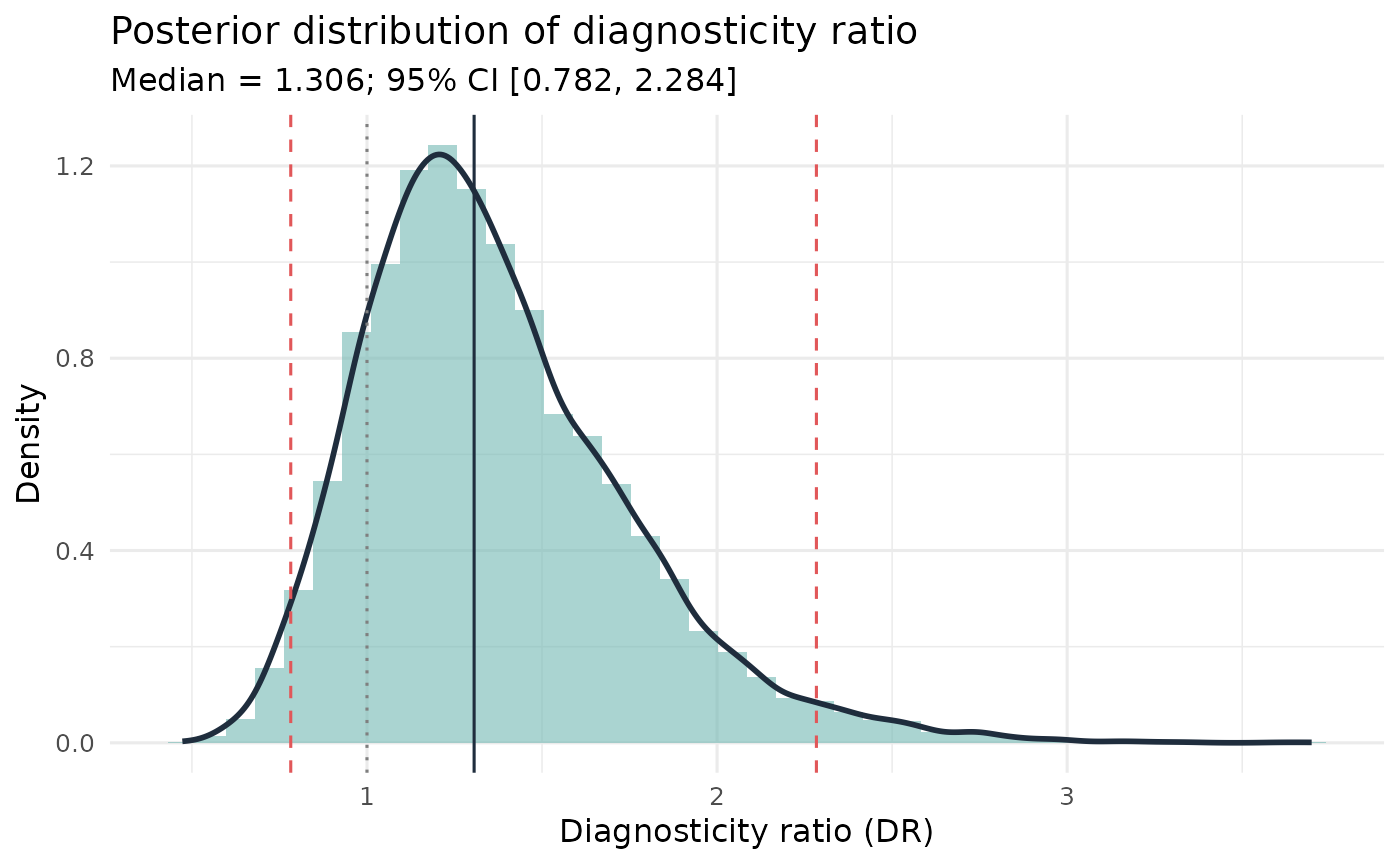
The target-present suspect-selection rate $p_{TP}$ and the target-absent rate $p_{TA}$ are modelled independently with Beta posteriors: $$p_{TP} \mid \mathbf{n} \sim \mathrm{Beta}(n_{TP,s} + \alpha,\; N_{TP} - n_{TP,s} + \alpha)$$ $$p_{TA} \mid \mathbf{n} \sim \mathrm{Beta}(n_{TA,s} + \alpha,\; N_{TA} - n_{TA,s} + \alpha)$$ The posterior of the diagnosticity ratio is obtained by drawing $DR^{(s)} = p_{TP}^{(s)} / p_{TA}^{(s)}$ for each sample $s$. The default Jeffreys prior ($\alpha = 0.5$) is recommended for small samples. Unlike the continuity-corrected point estimate, the posterior handles zero cell counts naturally and provides direct probability statements such as $P(DR > 1 \mid \mathbf{n})$.

The posterior mean is computed exactly, not from the draws. Because the two rates are independent, $E[DR] = E[p_{TP}] \, E[1/p_{TA}]$, with $E[1/p_{TA}] = (a + b - 1)/(a - 1)$ for $p_{TA} \sim \mathrm{Beta}(a, b)$ when $a > 1$. When $a \le 1$ (for example, no target-absent suspect choices under the Jeffreys prior) the mean is infinite, and an average of the draws would not settle on any value as S grew. Report the median and interval instead. In diag_ratio_T_bayes_compare(), the mean difference is NA when both means are infinite.

References

Tredoux, C. G. (1998). Statistical inference on measures of lineup fairness. Law and Human Behavior, 22(2), 217-237.

Wells, G. L., & Turtle, J. W. (1986). Eyewitness identification: The importance of lineup models. Psychological Bulletin, 99(3), 320-329.

Examples

set.seed(1)
lineup_pres <- round(runif(100, 1, 6))
lineup_abs  <- round(runif(80, 1, 6))
res <- diag_ratio_T_bayes(lineup_pres, lineup_abs, pos_pres = 3, pos_abs = 3,
                           k1 = 6, k2 = 6)
print(res)
#> Bayesian Diagnosticity Ratio (Tredoux) - Beta-Binomial model
#>   Prior: Jeffreys-type Beta(0.50, 0.50)
#>   TP lineup: n = 100, suspect IDs = 28
#>   TA lineup: n = 80, suspect IDs = 17
#>   Posterior mean DR:   1.368
#>   Posterior median DR: 1.306
#>   95% credible interval: [0.782, 2.284]
plot(res)