Bayesian Comparison of Effective Size (Tredoux, 1998) Across Two Lineups

Fits independent Dirichlet-Multinomial models to two lineup tables and returns the posterior distribution of the difference in Tredoux E'.

Usage

esize_T_bayes_compare(
  table_a,
  table_b,
  alpha = 0.5,
  S = 10000,
  credible_mass = 0.95
)

Arguments

table_a: A table of choice counts for lineup A.
table_b: A table of choice counts for lineup B.
alpha: Dirichlet concentration parameter(s). Applied to both lineups. A scalar or a length-k vector (both lineups must have the same k). Default 0.5 (Jeffreys).
S: Number of posterior draws per lineup. Default 10000.
credible_mass: Width of the equal-tailed credible interval for the difference. Default 0.95.

Value

An object of class "esize_T_bayes_compare" containing:

delta: Posterior draws of Delta = E'_A - E'_B.
posterior_mean: Posterior mean of Delta.
posterior_median: Posterior median of Delta.
credible_interval: Named 2-vector (lower, upper) for Delta.
P_A_greater: Posterior probability that E'_A > E'_B.
P_B_greater: Posterior probability that E'_B > E'_A.
result_a: The esize_T_bayes object for lineup A.
result_b: The esize_T_bayes object for lineup B.
credible_mass: Credible interval width.
S: Number of posterior draws.

Details

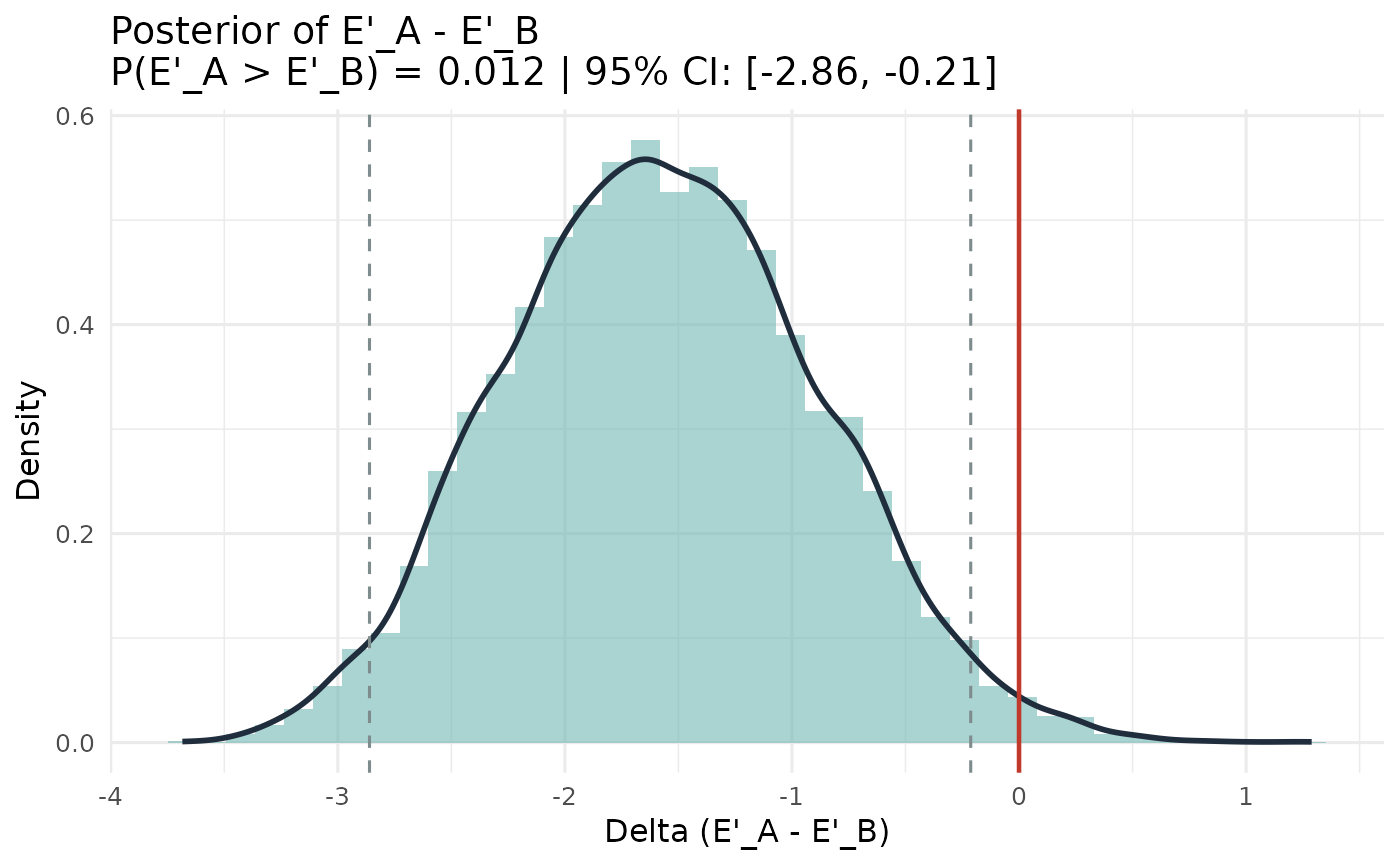
Independent Dirichlet-Multinomial posteriors are fitted for each lineup. The posterior of Delta = E'_A - E'_B is obtained by subtracting corresponding draws. P(E'_A > E'_B | data) is reported directly.

When the two lineups have different nominal sizes (different k), alpha must be a scalar; it is expanded independently for each lineup.

References

Tredoux, C. G. (1998). Statistical inference on measures of lineup fairness. Law and Human Behavior, 22(2), 217-237.

Examples

counts_a <- c(20, 5, 5, 5, 5, 5)
counts_b <- c(10, 8, 8, 8, 8, 8)
tab_a <- as.table(setNames(counts_a, 1:6))
tab_b <- as.table(setNames(counts_b, 1:6))

result <- esize_T_bayes_compare(tab_a, tab_b)
print(result)
#> Bayesian Comparison: Effective Size E' (Tredoux, 1998), A vs B
#> -----------------------------------------------------------
#>   Lineup A: k = 6, N = 45   |   Lineup B: k = 6, N = 50
#>   S (draws): 10000    Prior: Dirichlet(alpha = 0.50)
#>   E'_A posterior median: 3.904
#>   E'_B posterior median: 5.526
#>   Delta (E'_A - E'_B) posterior mean:   -1.571
#>   Delta posterior median:               -1.588
#>   95% credible interval for Delta: [-2.860, -0.213]
#>   P(E'_A > E'_B | data): 0.012
#>   P(E'_B > E'_A | data): 0.988
plot(result)