Multi-d' Model of Lineup Performance (Lee & Penrod, 2019)

Computes the multiple empirical discriminability (d') indices of Lee and Penrod's (2019) Multi-d' model from target-present (TP) and target-absent (TA) lineup data. Unlike the conventional 2 x 2 signal detection treatment, which folds filler identifications into "negative" responses, the Multi-d' model uses the full 2 x 3 response table (suspect ID, filler ID, rejection) in each lineup type.

Usage

make_multid(
  data = NULL,
  counts = NULL,
  lineup_size = 6,
  filler_rate = c("total", "per_filler"),
  correction = c("loglinear", "half", "none"),
  by_confidence = FALSE,
  conf_thresholds = NULL,
  n_bootstrap = 0,
  conf_level = 0.95,
  seed = NULL,
  innocent_suspect = "auto"
)

Arguments

data: A data frame with columns target_present (logical) and identification ("suspect", "filler" or "reject"). A confidence column is needed only when by_confidence = TRUE. TA rows with identification == "suspect" mark a designated innocent suspect; if there are none, the innocent suspect is estimated from filler choices (see Details). Supply either data or counts.
counts: A named numeric vector of response frequencies with elements G (guilty-suspect IDs), Fp (TP filler IDs), Rp (TP rejections), I (innocent-suspect IDs), Fa (TA filler IDs) and Ra (TA rejections). Omit I (or set it to NA) when the TA lineups have no designated innocent suspect; Fa is then the total number of TA filler IDs and is split as described in Details. Proportions may be supplied in place of frequencies, provided n_bootstrap = 0.
lineup_size: Nominal lineup size (suspect plus fillers). Default 6.
filler_rate: Either "total" (default), which uses the total filler ID rate as Lee and Penrod (2019) do, or "per_filler", which divides each filler ID rate by the number of fillers (lineup_size - 1) so that the filler indices refer to an average single filler.
correction: Correction for rates of 0 or 1: "loglinear" (default), "half" or "none". See sdt_summary_from_counts. Use "none" to reproduce published values computed from raw proportions.
by_confidence: Logical. If TRUE, the indices are also computed cumulatively by confidence, as in Lee and Penrod's (2019) Table 9. Requires data with a confidence column.
conf_thresholds: Optional numeric vector of confidence thresholds for by_confidence. Defaults to every observed confidence value.
n_bootstrap: Number of bootstrap resamples for percentile confidence intervals (default 0, no bootstrap). Resampling is done within the TP and TA arms separately.
conf_level: Confidence level for bootstrap intervals. Default 0.95.
seed: Optional random seed for the bootstrap.
innocent_suspect: For trial-level data, how innocent-suspect identifications are obtained; see make_rocdata. Ignored for counts, where the presence of I decides.

Value

An object of class "multid", a list with:

indices: Data frame of indices with estimates and, if bootstrapped, standard errors and percentile confidence limits.
rates: Named vector of the six response rates used (after correction and, if requested, per-filler scaling).
counts: Named vector of the six response counts (after any average-filler split).
n_tp, n_ta: Number of TP and TA lineups.
innocent_method: "designated" or "estimated_from_fillers".
by_confidence: Data frame of cumulative indices by confidence threshold, or NULL.
boot: Matrix of bootstrap draws, or NULL.

plus the settings used.

Details

With each d' computed as the difference between two z-transformed (inverse-normal) response rates, the model defines:

$d'(GI) = z(G) - z(I)$: guilty versus innocent suspect, the usual empirical discriminability;
$d'(GFp) = z(G) - z(Fp)$: guilty suspect versus TP fillers;
$d'(IFa) = z(I) - z(Fa)$: innocent suspect versus TA fillers, which Lee and Penrod treat as TA lineup bias;
$d'(FaFp) = z(Fa) - z(Fp)$: the greater appeal of TA than TP fillers (differential filler siphoning);
$d'(RaRp) = z(Ra) - z(Rp)$: discrimination of culprit presence from culprit absence (detection).

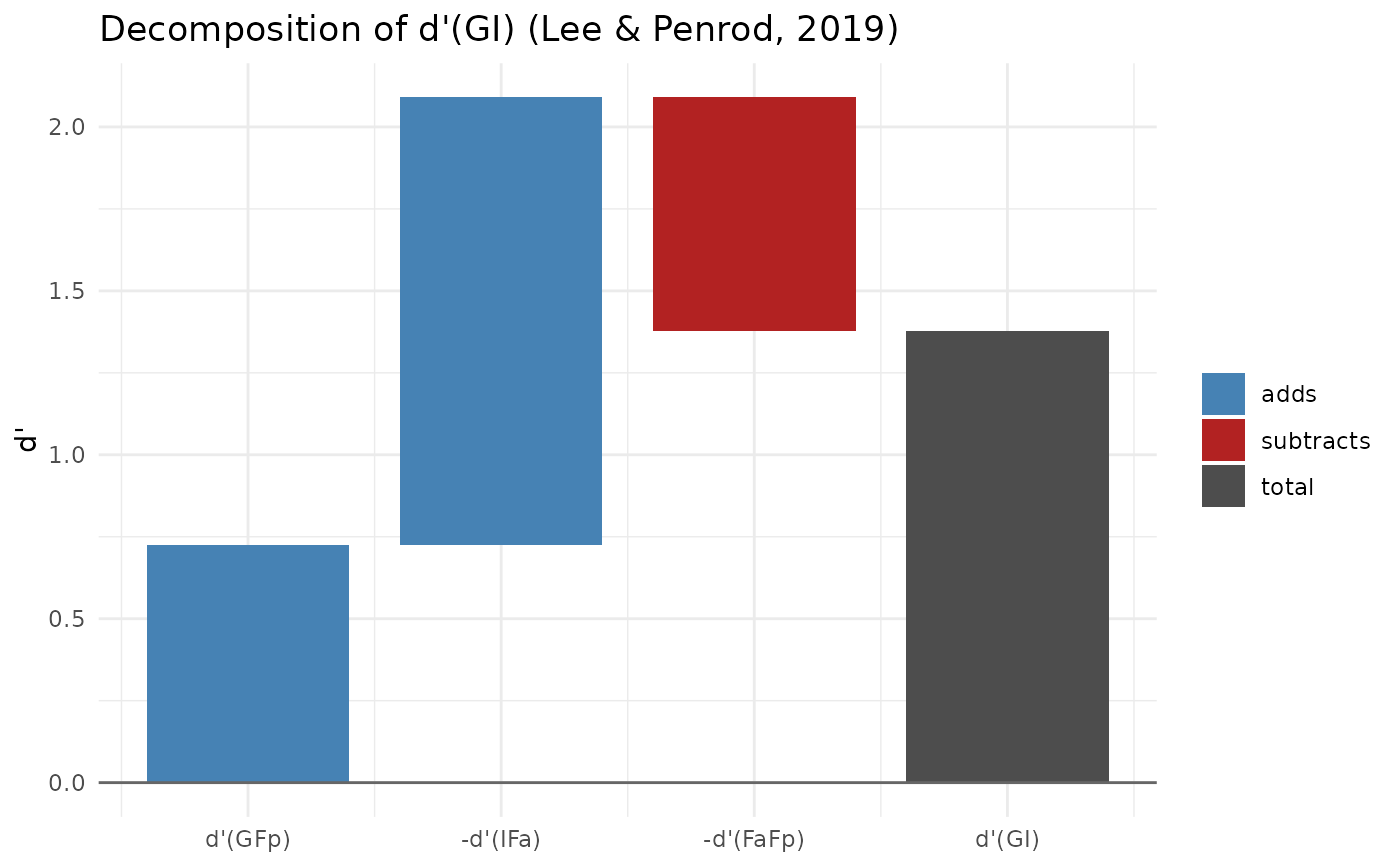
Lee and Penrod also propose $d'(GFp) - d'(RaRp)$ as an index of TP lineup bias net of memory strength, and $d'(GFp) - d'(IFa)$ as an index of differential filler siphoning. The decomposition $$d'(GI) = d'(GFp) - d'(IFa) - d'(FaFp)$$ holds exactly for any data, because the filler terms cancel. It is an accounting identity that shows where d'(GI) comes from, not an empirical result.

When TA lineups have no designated innocent suspect, the innocent-suspect count is estimated as the TA filler count divided by lineup_size, and the remaining $(k - 1)/k$ of filler choices are kept as TA filler IDs. Lee and Penrod call this the "average-filler" practice. It forces the TA lineup to be fair, so d'(IFa) then reflects the rejection rate rather than lineup bias.

With filler_rate = "total", a perfectly fair TA lineup does not give $d'(IFa) = 0$: the innocent suspect is compared with all fillers together. The returned fair_reference is the d'(IFa) a perfectly fair lineup would give at the observed TA rejection rate (for example, about -1.93 when no one rejects a 6-person lineup), and ifa_vs_fair is the observed d'(IFa) minus that reference. These two quantities are not part of Lee and Penrod's model; they are provided to help interpret d'(IFa). With filler_rate = "per_filler", the fair reference is 0, and the average-filler practice gives d'(IFa) = 0 exactly when correction = "none" (a rate correction shifts the two rates slightly differently).

The criterion c is $-(z(G) + z(I))/2$ and dr is the diagnosticity ratio G/I, both as reported by Lee and Penrod (2019).

References

Lee, J., & Penrod, S. D. (2019). New signal detection theory-based framework for eyewitness performance in lineups. Law and Human Behavior. doi:10.1037/lhb0000343

Lee, J., Mansour, J. K., & Penrod, S. D. (2022). Validity of mock-witness measures for assessing lineup fairness. Psychology, Crime & Law. doi:10.1080/1068316X.2021.1905811

Lee, J., Mansour, J. K., & Penrod, S. D. (2024). How to measure lineup fairness: Concurrent and predictive validity of lineup-fairness measures. Psychology, Crime & Law. doi:10.1080/1068316X.2024.2307358

Examples

# Lineup column of Lee & Penrod's (2019) Table 4 (Steblay et al., 2003)
md <- make_multid(counts = c(G = 45, Fp = 24, Rp = 31, I = 17, Fa = 26, Ra = 57),
                  correction = "none")
md
#> Multi-d' model (Lee & Penrod, 2019)
#>   TP lineups: 100   TA lineups: 100   Lineup size: 6
#>   Innocent suspect: designated   Filler rate: total   Correction: none
#> 
#> Response rates:
#>    G   Fp   Rp    I   Fa   Ra 
#> 0.45 0.24 0.31 0.17 0.26 0.57 
#> 
#>                                        description estimate
#>                 d'(GI): guilty vs innocent suspect     0.83
#>              d'(GFp): guilty suspect vs TP fillers     0.58
#>  d'(IFa): innocent suspect vs TA fillers (TA bias)    -0.31
#>                   d'(FaFp): TA vs TP filler appeal     0.06
#>              d'(RaRp): culprit presence vs absence     0.67
#>                 d'(GFp) - d'(RaRp): TP lineup bias    -0.09
#> 
#> Decomposition: d'(GI) = d'(GFp) - d'(IFa) - d'(FaFp): 0.83 = 0.58 - (-0.31) - (0.06)
#> Fair-lineup reference for d'(IFa): -1.10 (observed minus reference: 0.79)

# From trial-level data, with bootstrap CIs and confidence breakdown
data(lineup_example)
md2 <- make_multid(lineup_example, by_confidence = TRUE,
                   n_bootstrap = 200, seed = 1)
summary(md2)
#> Multi-d' model (Lee & Penrod, 2019)
#>   TP lineups: 700   TA lineups: 700   Lineup size: 6
#>   Innocent suspect: designated   Filler rate: total   Correction: loglinear
#> 
#> Response rates:
#>     G    Fp    Rp     I    Fa    Ra 
#> 0.593 0.312 0.096 0.126 0.587 0.287 
#> 
#>                                        description estimate    se ci_lower
#>                 d'(GI): guilty vs innocent suspect    1.379 0.082    1.192
#>              d'(GFp): guilty suspect vs TP fillers    0.726 0.092    0.525
#>  d'(IFa): innocent suspect vs TA fillers (TA bias)   -1.364 0.094   -1.548
#>                   d'(FaFp): TA vs TP filler appeal    0.711 0.073    0.575
#>              d'(RaRp): culprit presence vs absence    0.742 0.086    0.590
#>                 d'(GFp) - d'(RaRp): TP lineup bias   -0.017 0.122   -0.258
#>  ci_upper
#>     1.522
#>     0.885
#>    -1.175
#>     0.861
#>     0.909
#>     0.194
#> 
#> Decomposition: d'(GI) = d'(GFp) - d'(IFa) - d'(FaFp): 1.379 = 0.726 - (-1.364) - (0.711)
#> Fair-lineup reference for d'(IFa): -1.419 (observed minus reference: 0.054)
#> 
#> All indices:
#>           index estimate    se ci_lower ci_upper
#>              GI    1.379 0.082    1.192    1.522
#>             GFp    0.726 0.092    0.525    0.885
#>             IFa   -1.364 0.094   -1.548   -1.175
#>            FaFp    0.711 0.073    0.575    0.861
#>            RaRp    0.742 0.086    0.590    0.909
#>         tp_bias   -0.017 0.122   -0.258    0.194
#>       siphoning    2.090 0.139    1.822    2.355
#>  fair_reference   -1.419 0.024   -1.467   -1.373
#>     ifa_vs_fair    0.054 0.090   -0.115    0.240
#>               c    0.455 0.035    0.386    0.516
#>              dr    4.695 0.499    3.741    5.703
#> 
#> Cumulative indices by confidence (responses at or above threshold):
#>  threshold     G    Fp    Rp     I    Fa    Ra    GI   GFp    IFa  FaFp  RaRp
#>        100 0.098 0.011 0.001 0.001 0.029 0.001 1.895 1.006 -1.297 0.409 0.000
#>         90 0.143 0.019 0.001 0.006 0.044 0.001 1.423 1.004 -0.777 0.358 0.000
#>         80 0.189 0.039 0.001 0.015 0.065 0.001 1.289 0.878 -0.656 0.245 0.000
#>         70 0.260 0.076 0.001 0.024 0.128 0.001 1.343 0.788 -0.848 0.293 0.000
#>         60 0.352 0.109 0.001 0.031 0.180 0.001 1.490 0.850 -0.957 0.318 0.000
#>         50 0.436 0.163 0.001 0.055 0.270 0.001 1.437 0.819 -0.987 0.369 0.000
#>         40 0.507 0.218 0.001 0.078 0.369 0.001 1.438 0.798 -1.085 0.445 0.000
#>         30 0.556 0.265 0.001 0.103 0.479 0.001 1.402 0.769 -1.209 0.575 0.000
#>         20 0.593 0.312 0.096 0.126 0.587 0.287 1.379 0.726 -1.364 0.711 0.742
#>      c      dr
#>  2.242 137.000
#>  1.777  22.333
#>  1.526  12.619
#>  1.314  11.061
#>  1.126  11.465
#>  0.880   7.935
#>  0.701   6.523
#>  0.561   5.372
#>  0.455   4.695
plot(md2)