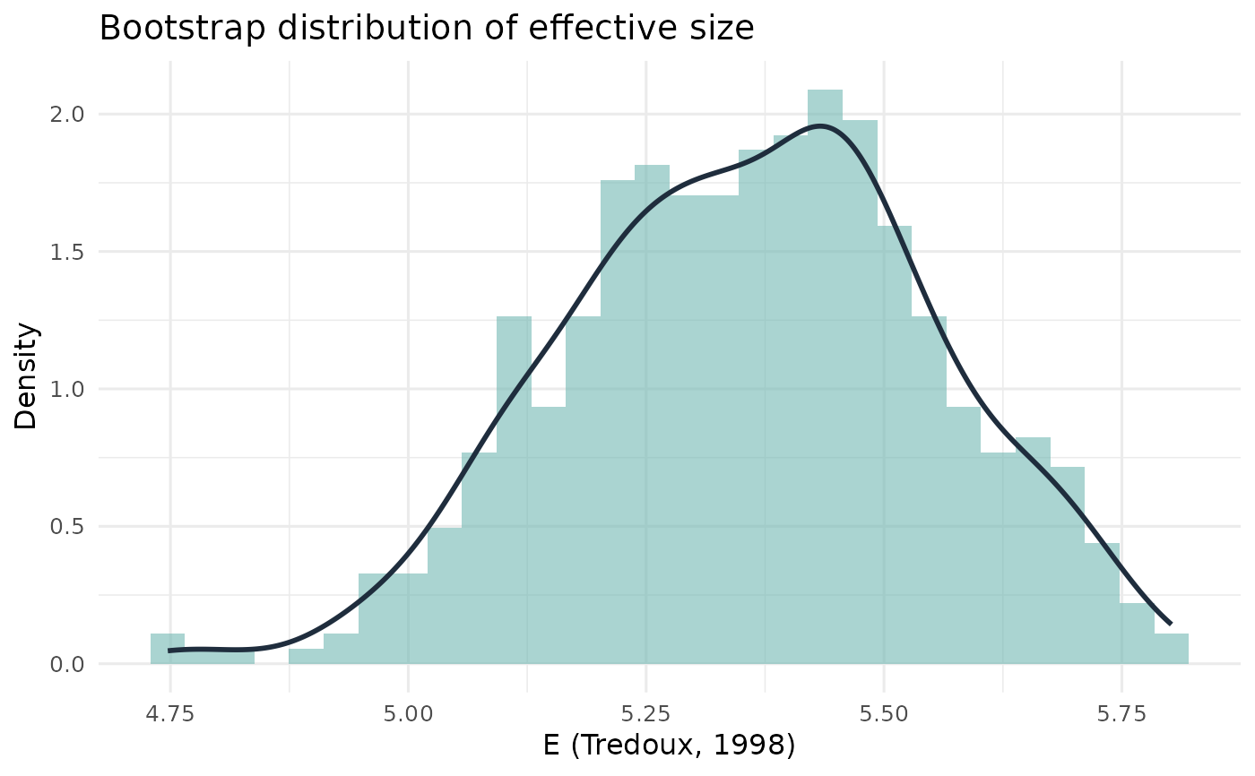
Plot Bootstrap Distribution of Effective Size

Usage

plot_esize_distribution(
  boot_values,
  metric = "Effective size",
  bins = NULL,
  binwidth = NULL
)

Arguments

boot_values: Numeric vector of bootstrap estimates, as returned by esize_boot_dist.
metric: Label for the effective size statistic.
bins: Number of histogram bins. Defaults to NULL, which selects the bin width automatically.
binwidth: Histogram bin width. Defaults to NULL, which selects the bin width automatically. Takes precedence over bins.

Value

A ggplot object.

Details

Effective size is a function of the whole table of choices, so its bootstrap distribution is usually fine-grained enough to bin as a continuous quantity, and the default is then 30 bins. When the number of lineup choices is small the estimates become visibly discrete, and the automatic rule bins at the resolution of the attainable values instead. See plot_lineup_bias_distribution for the rationale.

Examples

vec <- round(runif(200, 1, 6))
dist <- esize_boot_dist(vec, k = 6, metric = "tredoux", R = 500)
plot_esize_distribution(dist, metric = "E (Tredoux, 1998)")