Bayesian Comparison of SDT Sensitivity (d') Between Two Conditions

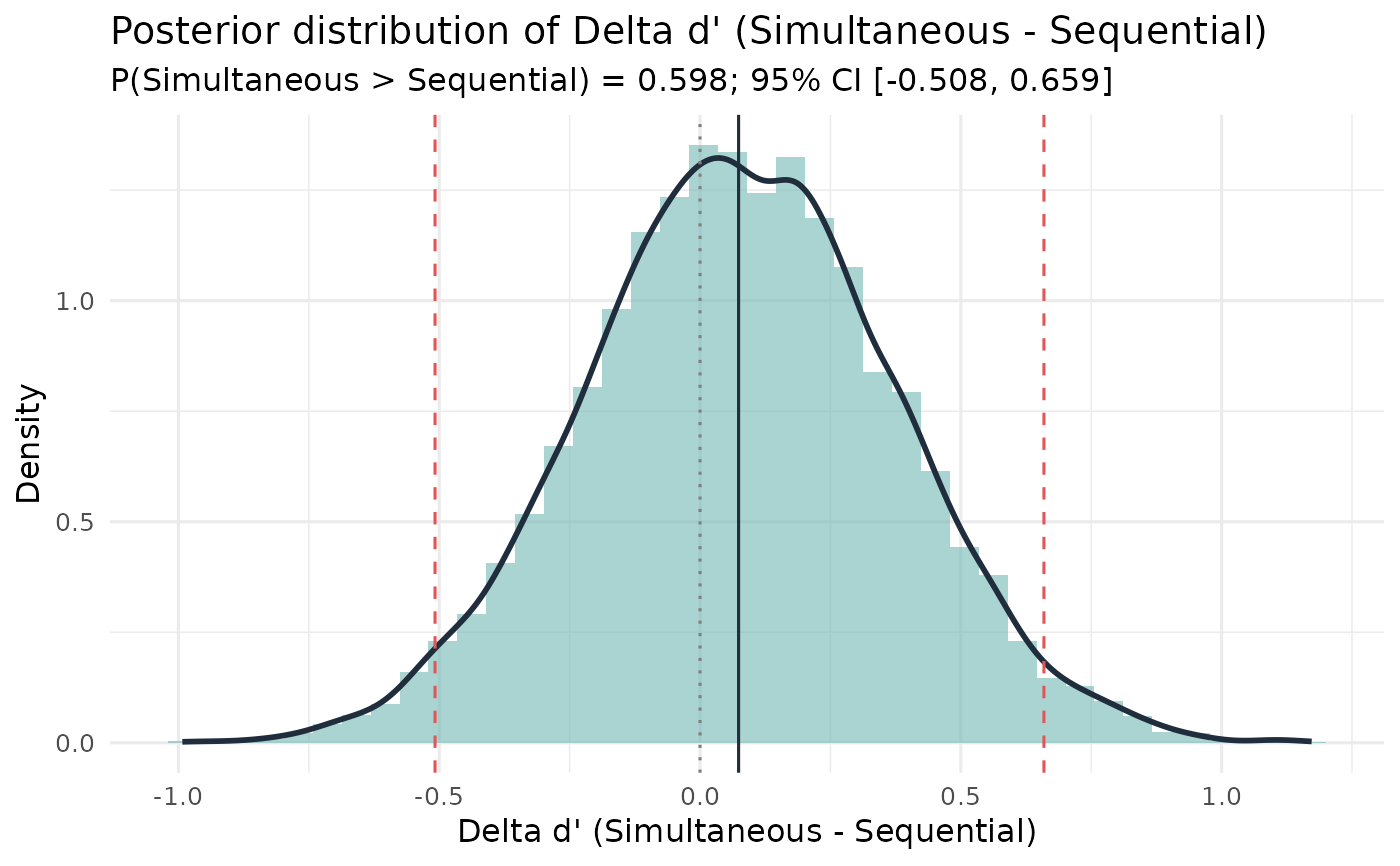
Computes a Bayesian posterior distribution for the difference \(\Delta d' = d'_A - d'_B\) using independent Jeffreys Beta posteriors for the hit and false-alarm rates in each condition.

Usage

sdt_compare(
  hits_A,
  misses_A,
  fas_A,
  crs_A,
  hits_B,
  misses_B,
  fas_B,
  crs_B,
  label_A = "A",
  label_B = "B",
  alpha = 0.5,
  S = 10000,
  credible_mass = 0.95
)

Arguments

hits_A, misses_A, fas_A, crs_A

Integer counts for condition A.

hits_B, misses_B, fas_B, crs_B

Integer counts for condition B.

label_A, label_B

Character labels for conditions (default "A", "B").

alpha

Prior concentration for the Beta prior on each rate. Default 0.5 (Jeffreys). Named shortcuts: "jeffreys", "uniform", "weak".

S

Number of posterior draws. Default 10000.

credible_mass

Width of the equal-tailed credible interval. Default 0.95.

Value

An object of class "sdt_compare" containing:

delta_dprime_draws

Posterior draws of \(\Delta d'\).

dprime_A_draws, dprime_B_draws

Per-condition d' draws.

posterior_mean, posterior_median

Posterior summaries of \(\Delta d'\).

credible_interval

Named lower/upper CI on \(\Delta d'\).

P_A_greater

Posterior probability that \(d'_A > d'_B\).

P_B_greater

Posterior probability that \(d'_B > d'_A\).

dprime_A_mean, dprime_B_mean

Posterior means of each d'.

frequentist

Output of compare_sdt_summary() for comparison.

prior_alpha, S, credible_mass

Metadata.

Details

Independent Jeffreys Beta posteriors are placed on the hit and false-alarm rates in each condition: $$HR_A \mid \mathbf{n} \sim \mathrm{Beta}(\text{hits}_A + \alpha,\; \text{misses}_A + \alpha)$$ $$FAR_A \mid \mathbf{n} \sim \mathrm{Beta}(\text{fas}_A + \alpha,\; \text{crs}_A + \alpha)$$ The posterior d' draws are: $$d'^{(s)}_A = \Phi^{-1}(HR_A^{(s)}) - \Phi^{-1}(FAR_A^{(s)})$$ and analogously for B. The posterior of the difference is \(\Delta d'^{(s)} = d'^{(s)}_A - d'^{(s)}_B\), from which \(P(d'_A > d'_B \mid \mathbf{n})\) is directly read off.

The Jeffreys prior (\(\alpha = 0.5\)) handles zero cell counts gracefully and provides direct probability statements - unlike the asymptotic z-test in compare_sdt_summary.

References

Macmillan, N. A., & Creelman, C. D. (2005). Detection Theory: A User's Guide (2nd ed.). Lawrence Erlbaum.

Wixted, J. T., & Mickes, L. (2014). A signal-detection-based diagnostic-feature detection model of eyewitness identification. Psychological Review, 121(2), 262-276.

See also

compare_sdt_summary, sdt_summary_from_counts, diag_ratio_T_bayes

Examples

# Simultaneous vs. sequential lineup comparison
res <- sdt_compare(
  hits_A = 45, misses_A = 55, fas_A = 12, crs_A = 88,
  hits_B = 38, misses_B = 62, fas_B = 10, crs_B = 90,
  label_A = "Simultaneous", label_B = "Sequential"
)
print(res)
#> Bayesian SDT Comparison: Simultaneous vs Sequential
#>   Prior: Jeffreys Beta(0.50, 0.50) on HR and FAR
#>   Posterior mean d': Simultaneous = 1.049, Sequential = 0.972
#>   Delta d' (Simultaneous - Sequential):
#>     Posterior mean:   0.077
#>     Posterior median: 0.074
#>     95% CI: [-0.508, 0.659]
#>   P(d'_Simultaneous > d'_Sequential | data): 0.5984
#>   P(d'_Sequential > d'_Simultaneous | data): 0.4016
#>   (Frequentist z-test: z = 0.254, p = 0.7994)
plot(res)